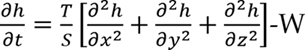
A classic example of a steady-state analytical model is recharge to a strip of land between two fully penetrating bodies of water. It simplifies flow in an unconfined aquifer by assuming the recharge is instantaneously and evenly distributed vertically throughout the aquifer and flow is horizontal within the aquifer.
The top boundary has steady, uniform recharge.
The two vertical boundaries are constant head. The water levels can be any height, but it is useful to remember that they represent fully penetrating water bodies so should fall within reasonable limits. The water level can be higher on the left or the right. If the water levels are very different and the distance between them is short, then the assumption of of essentially horizontal is not as reasonable. The further one deviates from the fundamental assumptions, the less accurate the model results.
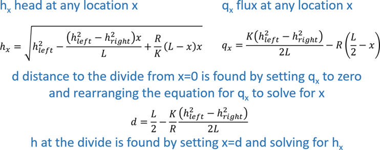
Given a value of recharge, hydraulic conductivity, head in each water body, and the distance between the water bodies, the model describes steady, one-dimensional, flow in a homogeneous porous material. Because the model is one-dimensional and steady state, it solves for:
head at any distance, x, from the left boundary, and
flow rate at any distance, x, from the left boundary.
The algebraic model presented here is founded on the the governing partial differential equation for flow, based on Darcy's Law and Conservation of Mass.
The symbols are: h=head, t=time, T=transmissivity, S=storativity, W=sources/sinks, and x,y,z are 3-D Cartesian coordinates. For WTR the equation is simplified to represent steady, one-dimensional flow in the x direction. It approximates unconfined conditions by ignoring the slope of the water table and assuming recharge is instantaneously distributed vertically throughout the aquifer, and water flows horizontally to water bodies of constant level on each side of the system.
The WTR equations are developed by Fetter (2001) in section 4.14, titled "Steady Flow in an Unconfined Aquifer" of his Applied Hydrogeology book, Prentice Hall, New Jersey, USA, 598 pages.
The algebraic equations are shown here, where R is the Recharge rate, K the hydraulic conductivity, L the length between water bodies (as shown in the image above).
Analytical models describing groundwater water levels and flow are mathematical models involving direct solution of the governing partial differential equations for flow for a specific aquifer geometry and associated boundary conditions. Generally, analytical flow models are limited to representing homogeneous materials in one or two dimensions using rectangular or radial coordinate systems.
Analytical models provide an exact, continuous, solution for head and/or flow as a function of space and, in the case of transient models, time. A continuous solution is one that can calculate a value for any location in space and time within the model domain (e.g., h at the location x=64.56 m after pumping a well for 5 minutes and 33 seconds). This is a distinct difference from numerical models which calculate values of head and flow at specific, predetermined, locations and times. When using a numerical model, the modeler interpolates between the resulting values to obtain heads and flows at locations and times between the calculated values. Numerical model values may be in error because the solution is iterative and did not close to a small tolerance or due to truncation of values of substantially different magnitude during the solution process. Given the precision and accuracy of analytical models, sometimes they are used to check if a newly developed numerical groundwater code produces accurate results.However, analytical models are limited to homogenous media with simple geometry and boundary conditions.