0. Introduction

Analytical Groundwater Modeling: Theory and Applications Using Python. Jupyter Book Edition.
Mark Bakker and Vincent Post

0.00 Copyright, license, isbn, and doi

This book, except the cover, is © 2026, Mark Bakker and Vincent Post.
The cover image of this book is © 2026, Eva van Aalst, Mark Bakker, and Vincent Post.
This version of this book, except the cover, is licensed under Creative Commons “Attribution-NonCommercial-NoDerivatives 4.0 International” license CC BY-NC-ND 4.0.
ISBN: 978-1-77470-153-9.
doi: 10.62592/LZYP5793.

0.01 Preface

The importance of groundwater as a water supply source can hardly be overstated. Groundwater exists everywhere in the subsurface. Extraction of water from aquifers supports livelihoods, agriculture, and a variety of economic activities worldwide. Groundwater is an integral part of the hydrological cycle where it sustains ecosystems, such as wetlands and estuaries, and provides the base flow of streams and rivers of all sizes. The flow of water through the subsurface constitutes a major transport pathway for dissolved substances and plays a key role in the planetary cycle of many chemical elements.
      Groundwater resources have come under enormous stress in many parts of the world. Concerns over the quantity and quality of groundwater are the result of past and ongoing mismanagement. Overexploitation has resulted in significant lowering of water levels. Unsustainable pumping in coastal areas has resulted in seawater intrusion. And careless disposal and handling of chemicals at the land surface has resulted in contamination that threatens precious resources. Addressing these problems is possible only with adequate understanding of the flow in the subsurface.
      The investigation of groundwater systems relies first and foremost on measurements. Due to the difficulty and costs involved in obtaining these, data are commonly available at a few points only, which severely limits the knowledge of the three-dimensional system under investigation. It is sometimes possible to predict future developments based on measured time series, but it is rarely possible to make predictions from measured time series for new interventions in the system or when anthropogenic, environmental, or climatic changes alter the system’s response.
      Groundwater models are essential to gain an understanding of the behavior of groundwater systems and to evaluate management scenarios that cannot be tested at full scale in the field. Groundwater models, like all models, are simplified versions of a complex reality. It is an important skill for every modeler to decide how a system can be simplified without losing the essence. It is unfortunately often appealing to add complexity to models because it exists, even though it doesn’t affect the outcome significantly.
      The essence of a groundwater flow problem is captured in a set of equations called the mathematical model. Simple models can often be solved analytically. Before the advent of grid-based methods, groundwater solutions were necessarily simplified until they could be solved, for example by deriving an analytic solution to the mathematical model. Analytic solutions give insights into the flow of groundwater that is more difficult to obtain with grid-based solutions. It is often forgotten that analytic solutions have benefited from the advent of computer technology, just like grid-based methods. In particular, the development of high-level programming languages makes it easy to evaluate analytic solutions and visualize their results.
      Models play an important role in solving the formidable water problems of our planet, as they are used as instruments to better understand, manage, and protect our water resources. The authors hope that the knowledge contained in this book contributes to better groundwater models and, ultimately, better-informed management decisions in the future.

0.02 About this book

This book provides a fresh treatment of the fundamentals of groundwater flow and is intended as both training material for the next generation of university students and a useful resource for practitioners who want to refamiliarize themselves with the basics while simultaneously learning about the capabilities of Python. Programming skills were part of groundwater modeling in the early days of the personal computer age. Classic books from, e.g., Bear and Verruijt (1987) and Strack (1989) already included computer code (on paper or floppy disks), but that was before high-level computer languages such as Python conquered the world. The example programs developed in this book may serve as templates that can be modified and extended to simulate settings or processes not covered in this book. The focus is on the fundamentals of the quantitative methods used to simulate, understand, and solve groundwater problems.
      The premise of this book is that any groundwater modeler needs a fundamental understanding of the theory on which mathematical models of groundwater flow are based. Even when a modeler primarily makes grid-based models, it is important to understand the main approximations that form the basis of the mathematical model, their range of applicability, and the main consequences for the flow field. Insights into fundamental flow systems form the backbone of any good modeler. This book provides detailed descriptions of analytic solutions to many fundamental groundwater problems. Mathematical derivations are included for the simpler problems. The solutions to more complicated problems are presented without derivation, but their validity is verified.
      The structure of this book is such that the theoretical treatments of the modeling methods are exemplified by short pieces of Python computer code that demonstrate the implementation of the theory. Python is an open-source programming language that has rapidly gained popularity within science and engineering and is likely going to remain one of the most popular programming languages over the next decades. Its simple yet powerful syntax and interactive workflow make learning and using Python a breeze. The development of powerful packages for scientific computing and visualization has made it easier than ever to evaluate, explore, and visualize both simple and complicated groundwater solutions. Python is a great language to write scripts to evaluate groundwater models. Scripts may be combined with output and explanations (including mathematical equations) in Jupyter Notebooks, resulting in executable documents that are a full, transparent, and reproducible record of a model or analysis.
      All code examples presented in this book are available as Jupyter Notebooks from github., which facilitates easy exploration of the examples in this book. Even though the notebooks save the reader from having to do a lot of typing, there are important benefits to entering the code examples from the printed book into one’s own notebook or Python interpreter. As one types, one takes much better notice of the subtle details contained in the code fragments. Especially when errors occur, one is forced to analyze their cause, which may take some time, but at the reward of a deeper understanding and a more lasting learning experience. Therefore, novice students are particularly encouraged to use this method and not immediately trust that they understand the worked examples in the notebooks. Hands-on exercises are provided and commonly require short Python scripts to be solved. Numerical answers to selected exercises are included at the end of the book.
      This book starts with a brief introduction to the principles of groundwater flow. This chapter is assigned number 0 to remind the reader that Python uses a zero-based numbering system (and because of restrictions of Jupyter Book 1 it is given a special place in the table of contents). All other numbering in this book starts at 1. The remainder of this book consists of two parts, each consisting of five chapters. The first part concerns one-dimensional flow, while the second part concerns two-dimensional flow. A variety of flow systems are discussed, including confined, unconfined, semi-confined, and multi-aquifer flows. Both steady and transient flows are considered. Most examples include the evaluation of both the head and the flow, sometimes including travel times. Special attention is paid to interface flow in coastal aquifers.
      For each solution, at least three code blocks are presented. The first code block contains the parameter values used in the example. The second code block contains the solution. And the third code block contains a few basic commands to produce visual output, which resembles the presented figures. The visual output appears right below the third code block, or on the next page if the output does not fit on the page. The exact code to produce the final figures included in this book is not provided as it contains some detailed (and repetitive) commands to make the figures look nice for the book. For those groundwater engineers and hydrogeologists that are not familiar with Python programming, or need a refresher of some of the programming concepts, a short primer on Python programming is included in Appendix A of this book.

0.03 About the authors

Mark Bakker is a groundwater engineer and a professor at the faculty of Civil Engineering and Geosciences of the Delft University of Technology. He has taught groundwater and Python classes for more than two decades and is the originator and co-developer of many Python-based open-source modeling tools, including Timflow, Pastas, and Flopy.

Vincent Post is a hydrogeologist with research interests in coastal hydrogeology and groundwater quality. After a career in academia and research he founded Edinsi Groundwater in 2021. Python has become indispensable in his everyday professional life, and he actively promotes its use in hydrogeology by teaching courses and developing Python-based tools.

0.04 Preface to the Jupyter Book Edition

Groundwater always moves and so does technology. A lot has changed since we started writing this book ten years ago. The notebooks that formed the basis of the original 2022 book have been combined into a digital, interactive Jupyter Book. Several of the examples have been made interactive using sliders while others have been made into animations, so that readers can study the flow of groundwater without having to dive into Python right away. The Jupyter Book Edition has a few other improvements as compared to the original book: The answers to each exercise, whether it is a numerical or graphical answer, is provided directly below each exercise. The introduction of the complex potential is moved from Section 7.3 to the new Section 7.5 and is further only used in Section 7.6 and Chapter 10. Chapter 8 on the analytic element method is rewritten to use real variables only. Readers that want to do analytic elements using an (arguably more elegant) complex potential are referred to the original 2022 book. The notation of boundary conditions was changed slightly. A specified head on the left side of a domain is now called \(h_l\) and a specified head on the right side is called \(h_r\) (similarly for flux boundary conditions). This change was made to facilitate the use of these analytic solutions in the new book that we are working on called “Numerical Groundwater Modeling”. And finally, the few typographical errors that were found in the original 2022 book were corrected. To execute (and modify) the Python code in this book yourself, simply copy and paste it into your own Notebook or Python interpreter and run it there.

0.0 Basics of groundwater flow

Groundwater is defined as the water beneath the water table, where the pores are fully saturated with water. The flow of groundwater forms the subsurface part of the hydrological cycle. The main source of groundwater is precipitation (rain or snow) that reaches the water table after infiltrating into the soil. The resulting increase in groundwater volume is called recharge, sometimes called meteoric recharge to emphasize that the water originates from atmospheric precipitation.
      Natural groundwater discharge occurs where groundwater reaches the land surface, for example in springs, swamps, and wetlands, or directly into rivers, lakes, seas, or oceans. Shallow groundwater can also be extracted by vegetation or through evaporation directly at the soil surface. In many inhabited areas, significant amounts of water are extracted through pumping wells.

0.1 Hydraulic head

Groundwater may be reached by digging or drilling a hole in the ground. The level to which water rises in a borehole is called the hydraulic head, or simply the head. A piezometer is an observation well specifically designed to measure the head and consists of a pipe with a slotted screen at the bottom. The water level in a piezometer rises to a height such that the weight of the water column in the piezometer equals the pressure of the groundwater directly adjacent to the well screen. In a well-constructed piezometer (i.e., one that has no leaks or internal flow), the pressure distribution with depth is hydrostatic

(1)\[ p = \rho g (h - z) \]

where \(p\) [M/L/T\(^2\)] is the pressure with respect to the atmosphere in the groundwater at the elevation of the well screen, \(\rho\) [M/L\(^{3}\)] is the (mean) density of the water in the piezometer, \(g\) [L/T\(^2\)] is the gravitational acceleration, \(h\) [L] is the head, and \(z\) [L] is the elevation of the well screen (positive upward) with respect to a reference level. Equation ((1)) can be rewritten as (Figure 1)

(2)\[ h = z + \frac{p}{\rho g} \]

The term \(z\) is also referred to as the elevation head, and the term \(p/(\rho g)\) as the pressure head. The pressure \(p\) equals zero at the water table so that the hydraulic head is equal to the elevation head, \(h = z\). Comparing water levels from different wells requires all water levels to be expressed with respect to a common reference level or datum (e.g., mean sea level).

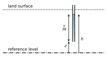
Figure 1 Definition of the head \(h\) and its components according to Eq. ((2)).

Exercise 1

Consider a piezometer of which the top is 20 m above the datum. The well screen is 30 m below the top of the piezometer. A pressure sensor is lowered into the piezometer to a depth of 10 m below the top of the piezometer and records an absolute pressure of \(p_\text{abs}=180\) kPa. The piezometer is filled with fresh water with a density \(\rho=1000\) kg/m\(^3\). Atmospheric pressure is measured to be 101 kPa. Use \(g=9.8\) m\(^2\)/s. Compute the head in the well.

Solution

\(h = 18.06\) m

0.2 Darcy’s experiment

In 1856, the French engineer Henry Darcy published the results of a series of experiments on the flow of water through a column packed with different kinds of sand (Darcy, 1856). The experiments consisted of a soil column of length \(L\) and cross-sectional area \(A\) (Figure 2). Darcy measured the discharge \(Q\) through the column and the difference \(\Delta h\) in the head of the water between two measurement ports.

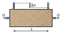
Figure 2 Schematic representation of Darcy’s experiment. Darcy used a vertical column, but a horizontal column works just as well.

      The experiments revealed that there is a linear relationship between the discharge \(Q\) through the soil column and the hydraulic head drop \(\Delta h\) over distance \(L\), which can be expressed as

(3)\[ Q = kA \frac{\Delta h}{L} \]

The proportionality constant \(k\) was introduced because the relationship between the discharge and the head gradient differed between types of sand. Nowadays, \(k\) is known as the hydraulic conductivity, which has the dimensions L/T. Darcy’s law is not a physical law, but an empirical relation. It became known as a law because it performs remarkably well over a large range of flow conditions.

0.3 Representative elementary volume

Water particles move through small openings in the subsurface, along convoluted pathways caused by the irregular shape of the pore space. The simulation of groundwater flow at this microscopic scale requires knowledge of the three-dimensional shape of the entire pore space, which is not feasible. A different approach is required for larger spatial scales, called the macroscopic scale. At the macroscopic scale, the net movement of groundwater through the subsurface is approximated using parameters that are a representative average of the behavior at the microscopic scale. This is what Darcy established empirically: The friction and viscous forces that work against the flow of water are captured by the hydraulic conductivity \(k\). This parameter thus represents the effective action of the processes at the microscopic scale, without detailed knowledge of the pore geometry at this scale.
      The variables for the macroscopic description of groundwater flow are associated with a spatial scale that is representative of the system considered. The volume for which a macroscopic property is valid is called the representative elementary volume (REV). The REV must not be too small, because it will not form a representative average. In the extreme, an REV smaller than the size of a pore or soil particle either represents an opening between soil particles or a soil particle itself, but not the average of many of these combined. The size of an REV must therefore exceed a multiple of the representative pore size. Conversely, an REV must not be too large either as it may no longer be suited to resolve the spatial variability of the subsurface at the macroscopic level. If the properties of the subsurface vary over a few meters, the REV must be significantly smaller than a few meters to capture this variability in a model. The REV relevant to practical groundwater problems varies. For unconsolidated sands, with a pore and grain size on the order of tenths of a millimeter, an REV of a few centimeters already captures the average behavior.

0.4 Hydraulic conductivity and porosity

The hydraulic conductivity \(k\) is a measure of how easy a fluid can flow through the subsurface. The hydraulic conductivity is not just a property of the subsurface, but also a property of the fluid that flows through the subsurface and may be written as

(4)\[ k = \frac{\kappa \rho g}{\mu} \]

where \(\kappa\) [L\(^2\)] is the intrinsic permeability that depends on the porous medium, while the density, \(\rho\), and the dynamic viscosity, \(\mu\) [M/L/T], are properties of the fluid that flows through the subsurface. This means that warmer water will have a higher hydraulic conductivity than colder water, even when it flows through the same subsurface, as the viscosity of warmer water is smaller than the viscosity of colder water. Typical values of the hydraulic conductivity of water through different materials are presented in Table 1.

Table 1 Hydraulic conductivity ranges of different materials

Material	\(k\) (m/d)
Clay	< 0.0001
Sandy clay	0.0001 – 0.001
Peat	0.0001 – 0.01
Silt	0.001 – 0.01
Very fine sand	0.1 – 1
Fine sand	1 – 10
Coarse sand	10 – 100
Sand with gravel	100 – 1000
Gravel	> 1000

Source: Modified from Verruijt (1970)

      The porosity, \(n\), of the subsurface is defined as the ratio of the volume of pores, \(V_{p}\), to the total volume, \(V_{t}\).

(5)\[ n = \frac{V_{p}}{V_{t}} \]

The porosity does not appear in the equation for the hydraulic conductivity (Eq. (4)), but the intrinsic permeability \(\kappa\) depends on the characteristics of the subsurface, including the pore volume, the pore size distribution, the connectivity between pores, the shape of the pores, and the roughness of the subsurface material. The porosity therefore partially determines the intrinsic permeability \(\kappa\) and thus indirectly influences \(k\) as well.

Exercise 2

Compute the hydraulic conductivity (in m/d) of freshwater flowing through sand in the winter when the infiltrating water has a temperature of 5 \(^\circ\)C and in the summer when infiltrating water has a temperature of 20 \(^\circ\)C. Given: \(\kappa=2\cdot 10^{-11}\) m\(^2\), \(\mu=1.5\cdot 10^{-3}\) Ns/m\(^2\) at 5 \(^\circ\)C, and \(\mu=1\cdot 10^{-3}\) Ns/m\(^2\) at 20 \(^\circ\)C.

Solution

\(k = 11.29\) m/d, \(k = 16.93\) m/d

0.5 Aquifers and aquitards

The subsurface consists of layers of varying permeability. The permeable layers are referred to as aquifers. Sediments such as sand or gravel tend to form good aquifers, as their pores are relatively wide and well connected, so that water can flow with relative ease. Layers with a lower permeability are called aquitards, leaky layers, or semi-confining layers. Truly impermeable layers do not exist in nature, but if the hydraulic conductivity is so low that flow through them is negligible, they are sometimes called aquicludes or confining layers.

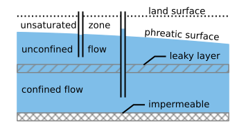
Figure 3 Schematic cross section of the subsurface showing aquifers and aquitards.

      An aquifer is unconfined when the saturated domain is bounded at the top by the water table, also called the phreatic surface (Figure 3). Confined aquifers are separated from other aquifers, or the land surface, by an aquitard. Flow is referred to as confined when the head is above the top of the aquifer (Figure 3). The head in confined aquifers can drop below the top of the aquifer, resulting in unconfined flow (see Section 3.3). Artesian conditions exist when the head in a confined aquifer is higher than the elevation of the land surface, which means that groundwater flows freely to the surface if a well is installed, without the need for a pump.
      In systems consisting of multiple aquifers separated by aquitards, groundwater may move from one aquifer to another through aquitards. This is referred to as multi-aquifer or inter-aquifer flow. Flow in aquitards can often be approximated as vertical. The larger the thickness of an aquitard, the more difficult it is for water to flow across it. The ratio of the thickness of an aquitard to its vertical hydraulic conductivity is called the hydraulic resistance and is a measure of the (im)permeability of a leaky layer. Flow in aquifers tends to be predominantly horizontal. The larger the thickness of an aquifer, the more water it can transmit. The ability of an aquifer to transmit water in the horizontal direction is called the transmissivity, which is the product of the hydraulic conductivity and the aquifer thickness.
      A groundwater modeler must always decide about the base of the groundwater flow system, which is commonly formed by a low-permeable layer that leaks so little water that it can be neglected for the problem of interest. While it is common to refer to the bottom of the system as the impermeable base, it must be realized that there is always some exchange of water across the bottom boundary of the system considered. Ideally, a confining unit can be defined that serves as the base of the model, and in this case, a better term for the base of the model is the basal aquitard. For very thick aquifer systems (like in sedimentary basins and deltas, which can be many kilometers deep), this is not always feasible, and a pragmatic choice must be made.

0.6 Storage and transient flow

When there are no significant changes in head (and thus flow) through time, the flow is said to be steady. Analyses of steady flow are appropriate when long-term, average conditions are of interest, for example for the delineation of wellhead protection areas for water supply wells, or when an end situation is of interest, as for the dewatering of an aquifer for a construction project. When the heads do not change with time, the storage volume remains constant in time, which implies that the inflow and outflow of water are equal in the system considered.
      In reality, groundwater flow is always transient. Transient flow occurs because boundary conditions and system stresses change through time, for example changing aquifer recharge, changing river levels, or varying pumping rates of wells. A specific application of transient flow analysis is the evaluation of aquifer properties by induced stresses, such as pumping tests.
      The storage in an unconfined aquifer increases when the water table rises. As an example, consider a column within an unconfined aquifer with constant horizontal cross-sectional surface area A. When the water table is raised \(\Delta h\), the volume of water in the column increases by an amount

(6)\[ \Delta V = S A \Delta h \]

where \(S\) [-] is the storativity or storage coefficient of the unconfined aquifer. When the porous medium above the water table is completely dry before the rise, the storativity of the unconfined aquifer is equal to the porosity. In reality, the storativity is always smaller than the porosity, as there is always soil water present above the water table. The storativity of an unconfined aquifer is referred to as the phreatic storage coefficient or the more cryptic specific yield and is represented by the variable \(S_p\). Typical values of the phreatic storage for different materials are presented in Table 2.

Table 2 Phreatic storage of different materials

Material	\(S_p\) (−)
Clay	0.01 – 0.05
Silt	0.03 – 0.19
Sand	0.1 – 0.35
Gravel	0.14 – 0.35

Source: Modified from Fitts (2013)

      Storage in a confined aquifer is physically more complicated. In a confined aquifer, all pores are entirely filled with water. Additional water can nevertheless be stored through expansion of the pore space and, albeit only to a small extent, compression of the water. When the head rises by \(\Delta h\), the volume of water increases by an amount \(\Delta V\) according to Eq. ((6)), but the storage coefficient is much smaller than that for unconfined aquifers. For most unconsolidated aquifers, the ability of the aquifer to expand is significantly larger than the ability of the water to compress. The storage coefficient of a confined aquifer is a function of the aquifer thickness: The thicker the aquifer, the more water can be stored per unit surface area \(A\), and thus the greater the storage coefficient. The storage coefficient of a confined aquifer is

(7)\[ S = S_s H \]

where \(S_s\) [1/L] is the specific storage of the aquifer (the storage per unit aquifer thickness) and \(H\) is the aquifer thickness. Typical values for the specific storage are presented in Table 3.

Table 3 Specific storage values for different materials

Material	\(S_s\) (m\(^{-1}\))
Clay	\(1 \cdot 10^{-3}\) – \(2 \cdot 10^{-2}\)
Sand	\(1 \cdot 10^{-5}\) – \(1 \cdot 10^{-3}\)

Source: Modified from Anderson et al. (2015)

0.7 Darcy’s law for groundwater modeling

The basic form of Darcy’s law (Eq. (3)) relates the total flow \(Q\) through a column of soil to the head gradient. For groundwater modeling, it is more useful to consider the discharge per unit area

(8)\[ q = \frac{Q}{A_q} = k \frac{\Delta h}{L} \]

where \(A_q\) is the cross-sectional area perpendicular to the flow. The dimensions of specific discharge are L/T. It is important to note, however, that the specific discharge is not a velocity (although it is sometimes confusingly referred to as the Darcy velocity), but a discharge per unit area.
      Groundwater flow can be in any direction and is expressed in terms of the specific discharge vector \(\vec{q}=(q_x, q_y, q_z)\) with components in each of the three coordinate directions. The general form of Darcy’s law relates the components of the specific discharge vector to the head gradient in each direction

(9)\[ q_x = -k\frac{\partial h}{\partial x} {\hskip 2em} q_y = -k\frac{\partial h}{\partial y} {\hskip 2em} q_z = -k\frac{\partial h}{\partial z} \]

      In Eq. ((9)), the hydraulic conductivity is the same for flow in all directions. In some aquifers, the hydraulic conductivity is anisotropic and must be represented by a tensor. When the principal directions of the hydraulic conductivity tensor coincide with the coordinate directions, Darcy’s law may be written as

(10)\[ q_x = -k_x\frac{\partial h}{\partial x} {\hskip 2em} q_y = -k_y\frac{\partial h}{\partial y} {\hskip 2em} q_z = -k_z\frac{\partial h}{\partial z} \]

where \(k_x\), \(k_y\), and \(k_z\) are the hydraulic conductivity in the three coordinate directions (the principal components of the hydraulic conductivity tensor).
      Water in the subsurface can only flow through the pores. The average velocity vector \(\vec{v}\) can be obtained from the specific discharge vector through division by the porosity \(n\)

(11)\[ \vec{v}=\frac{\vec{q}}{n} \]

The vector \(\vec{v}\) is the average velocity of the groundwater because it describes the flow at the macroscopic level, not the flow of individual water particles at the microscopic level of the pores.

Exercise 3

Compute the average groundwater velocity for sand with \(k=20\) m/d, a porosity of \(n=0.3\), and a head that drops 2 m every 1000 m. Compute \(v\) in both meters per day and meters per month.

Solution

\(v = 0.13\) m/d \(= 4.0\) m/month

0.8 Dupuit and Forchheimer

All groundwater flow is three-dimensional, but for modeling purposes, flow may be approximated as one-dimensional or two-dimensional. At the regional scale, most aquifers are relatively thin in comparison with their areal extent and are therefore referred to as shallow aquifers. Flow is predominantly horizontal in such aquifers and may be approximated as two-dimensional in the horizontal plane. The amount of horizontal flow is described by the discharge vector \(\vec{Q}=(Q_x,Q_y)\). The discharge vector is the total flow in the aquifer integrated over the saturated thickness \(H\) of the aquifer. In other words, it is the discharge per unit width of aquifer. The components of the discharge vector may be computed as

(12)\[ Q_x=Hq_x=-kH\frac{\partial h}{\partial x} {\hskip 2em} Q_y=Hq_y=-kH\frac{\partial h}{\partial y} \]

where the hydraulic conductivity is horizontally isotropic (\(k_x = k_y = k\)). The dimensions of the discharge vector are L\(^2\)/T. This approximation was first proposed by Dupuit (1863) and Forchheimer (1886), so it is referred to as Dupuit flow or Dupuit-Forchheimer flow.
      The Dupuit–Forchheimer approximation essentially means that the pressure distribution is hydrostatic in an aquifer. This is very convenient, because that means that the head \(h\) does not depend on the vertical coordinate in an aquifer. The Dupuit–Forchheimer approximation does not mean, however, that flow is horizontal. Water can still flow vertically, but the resistance to vertical flow is neglected within an aquifer; a detailed analysis is given in Chapter 1. The accuracy of the Dupuit–Forchheimer approximation is further explored in Chapter 10.

0.9 Groundwater models

Groundwater models are needed to gain an understanding of how groundwater flows and to try to make predictions, because most phenomena or proposed interventions cannot be tested at full scale in the field. Groundwater models are mathematical solutions to the differential equation that describes flow in an aquifer system. The differential equation is obtained through the combination of a mass balance equation and Darcy’s law, yielding a differential equation in terms of the hydraulic head. A mathematical model of a groundwater problem consists of a differential equation and a set of mathematical boundary conditions, which are derived from boundaries and conditions of the physical groundwater system. In this book, the mathematical problem is solved analytically.
      In each of the upcoming chapters, analytical solutions are presented for a wide range of flow problems. Chapters 1-5 deal with flow systems that may be approximated as one-dimensional in the horizontal direction. This is followed by solutions to two-dimensional flow systems in the horizontal plane in Chapters 6–9, including flow systems that are radially symmetric (e.g., flow near a pumping well). Finally, Chapter 10 deals with two-dimensional flow in the vertical plane, including a comparison with one-dimensional Dupuit–Forchheimer solutions.