7.2. Well capture zones

All water inside the capture zone envelope of a well is eventually captured by the well, but this can take a (very) long time. In groundwater management, it is important to delineate the zone that is captured by the well within a certain time period. For example, all the water in the 5-year capture zone reaches the well within 5 years. The capture zone for a certain time period can be computed by integrating time along a streamline from the well against the flow. For a single well in an otherwise uniform flow field, this can be done analytically, as was shown by Bear and Jacobs (1965). For more complicated settings, the integration is conducted numerically. In this section, the analytical solution is discussed first, followed by the numerical solution.
     Consider a well with discharge \(Q\) located at the origin in an otherwise uniform flow field with \(Q_x=U\) and \(Q_y=0\). The stream function for this problem is given by Eq. ((7.6)). The stream function equals zero along the capture zone envelope (see previous section), so that an equation for the capture zone envelope can be written as

(7.13)\[ \Psi = -Uy + \frac{Q}{2\pi}\theta = 0 \]

Using that \(y=r\sin\theta\) gives an expression for the radial distance from the well towards the capture zone envelope

(7.14)\[ r = \frac{Q}{2\pi} \frac{\theta}{U\sin(\theta)} \]

This means that for any angle \(\theta\), a distance \(r\) to the capture zone envelope can be computed with the above formula. The corresponding \(x,y\) coordinates of the capture zone envelope are computed with

(7.15)\[ x = r\cos(\theta) \hskip 2em y = r\sin(\theta) \]

The travel time \(t\) from location \((x,y)\) inside the capture zone envelope to the well can be computed with the following equation (Bear and Jacobs, 1965)

(7.16)\[ t = -\frac{nHx}{U} - \frac{QnH}{2\pi U^2} \ln\left[ \frac{ \sin(\theta - 2\pi U y / Q)}{\sin(\theta)} \right] \]

where \(H\) is the aquifer thickness and \(n\) is the porosity. In the example below, the travel time towards the well is computed for a number of points inside the capture zone envelope, after which the capture zones are obtained by contouring the travel times (Figure 7.4).

# parameters
n = 0.25 # porosity, -
k = 20 # hydraulic conductivity, m/d
H = 15 # aquifer thickness, m
dhdx = -0.002 # gradient, -
U = -k * H * dhdx # uniform flow, m^2/d
Q = 500 # discharge of the well, m^3/d
rw = 0.3 # radius of well, m

# solution
# coordinates of capture zone envelope
theta = np.linspace(-3, -1e-4, 100) # bottom half of envelope
r = Q / (2 * np.pi) * theta / (U * np.sin(theta))
xcap = r * np.cos(theta)
ycap = r * np.sin(theta)
# grid inside the capture zone envelope
xg = xcap * np.ones((50, len(xcap)))
yg = np.zeros_like(xg)
for i in range(len(xcap)):
    yg[:, i] = np.linspace(ycap[i] + 1e-3, -ycap[i] - 1e-3, 50)
# travel time for all grid points inside capture zone envelope
theta = np.arctan2(yg, xg)
tgrid = -n * H * xg / U - Q * n * H / (2 * np.pi * U ** 2) * np.log(
        np.sin(theta - 2 * np.pi * U * yg / Q) / np.sin(theta))

# basic capture zone plot
plt.subplot(111, aspect=1, xlim=(-1000, 150))
plt.plot(0, 0, 'k.')
plt.contourf(xg, yg, tgrid, [0, 5 * 362.25, 10 * 365.25]);

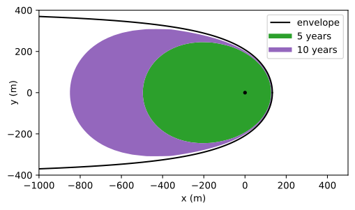
Figure 7.4 Capture zones for a well in a uniform background flow obtained with the analytic solution.

     Capture zones for more complicated settings, e.g. multiple wells or other boundary conditions, must be computed numerically as they can not be computed analytically. As was shown in the previous section, pathlines can be computed through numerical integration of the horizontal velocity vector (Eq. (7.12)). Pathlines can be traced against the flow in the same fashion by starting at the well and integrating the negative velocity vector (i.e., integrating against the flow).
     The following example concerns two wells in an otherwise uniform flow field in the \(x\)-direction. The discharge of both wells is equal to \(Q\). The 5-year capture zone is computed by starting 20 pathlines equally distributed along the circumference of each well. The pathlines are continued for 5 years against the flow (Figure 7.5).

# additional parameters
xw0, yw0 = 0, 0 # x,y-location well 0, m
xw1, yw1 = 100, 100 # x,y-location well 1, m
U = 1.2 # uniform flow in x-direction, m^2/d

# solution and plot
def minvxvy(t, xy): # function vxvy from Section 7.1
    x, y = xy
    rsq0 = (x - xw0)**2 + (y - yw0)**2
    rsq1 = (x - xw1)**2 + (y - yw1)**2
    Qx = U - Q / (2 * np.pi) * ((x - xw0) / rsq0 + (x - xw1) / rsq1)
    Qy = -Q / (2 * np.pi) * ((y - yw0) / rsq0 + (y - yw1) / rsq1)
    return np.array([-Qx, -Qy]) / (n * H)

from scipy.integrate import solve_ivp
xstart = rw * np.cos(np.arange(0, 2 * np.pi, np.pi / 10)) # spaced around well
ystart = rw * np.sin(np.arange(0, 2 * np.pi, np.pi / 10)) # spaced around well
plt.subplot(111, aspect=1)
for i in range(len(xstart)):
    path = solve_ivp(minvxvy, (0, 5 * 365), [xstart[i] + xw0, ystart[i] + yw0], 
                     t_eval=np.linspace(0, 5 * 365, 100))
    plt.plot(path.y[0], path.y[1], 'C1')
    path = solve_ivp(minvxvy, (0, 5 * 365), [xstart[i] + xw1, ystart[i] + yw1], 
                     t_eval=np.linspace(0, 5 * 365, 100))
    plt.plot(path.y[0], path.y[1], 'C2')

Figure 7.5 Five-year capture zones for two wells with equal discharge in a uniform background flow; pathlines are obtained through numerical integration.

Exercise 7.5

Compare the 5-year capture zone for the analytic solution of a single well in an otherwise uniform flow field to the capture zone obtained with the numerical procedure.

Solution

They are the same