5.3. Areal recharge between two rivers

The solution for steady recharge between two parallel rivers in an aquifer with constant transmissivity \(T\) that was presented in Section 1.2 is extended to include transient recharge. The rivers are a distance \(L\) apart; the origin of the coordinate system is chosen halfway between the two rivers (Figure 5.9). Initially, the head in the aquifer is at steady state, so the initial transient head equals zero. The rivers are in direct contact with the aquifer and the river stages are fixed so that the boundary conditions and initial condition of the transient head are

(5.39)\[ h\vert_{x=-L/2,t}=h\vert_{x=L/2,t}=h\vert_{x,t=0}=0 \]

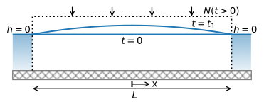
Figure 5.9 Transient recharge between two rivers (\(t_1>0\)).

     At time \(t=0\), areal recharge starts at a constant and uniform rate \(N\). The solution for the head in the aquifer as a function of time can be obtained with separation of variables and results in the following infinite series (Bruggeman, 1999, solution 133.16)

(5.40)\[ h = \frac{-N}{2T}\left(x^2 - \tfrac{1}{4}L^2\right) - \frac{4NL^2}{\pi^3T} \sum_{n=0}^\infty \frac{(-1)^n}{(2n + 1)^3} \cos\left[\frac{(2n+1)\pi x}{L}\right] \exp\left[-\frac{(2n+1)^2\pi^2 Tt}{SL^2}\right] \]

Note that for large times, the exponential term in the solution goes to zero and the head approaches the steady state solution \(\tfrac{-N}{2T}\left(x^2 - \tfrac{1}{4}L^2\right)\), which is Eq. ((1.24)) for the case that the heads in the river are set to zero and the origin of the coordinate system is halfway between the two rivers.
     In the following example, the head is plotted vs. \(x\) at three early times and at three late times and for a different number of terms in the series solution (Figure 5.10). For the early times, the solution is plotted using three terms in the series (dashed lines), which is not sufficient as a distinct wiggle is visible, especially for \(t=1\) d. For later times, the dashed solution represents only one term in the series solution, which is indistinguishable from the solution with ten or more terms.

# parameters
L = 1000 # aquifer length, m
S = 0.1 # storage coefficient, -
T = 200 # transmissivity, m^2/d
N = 0.001 # recharge rate, m/d

# solution
def head(x, t, T=T, S=S, L=L, N=N, nterms=10):
    h = 0
    for n in range(nterms):
        h += (-1)**n / (2 * n + 1)**3 * \
        np.cos(((2 * n + 1) * np.pi * x) / L) * \
        np.exp(-((2 * n + 1)**2 * np.pi**2 * T * t) / (S * L**2))
    h = -N / (2 * T) * (x**2 - L**2/4) - 4 * N * L**2 / (np.pi**3 * T) * h
    return h

# basic head plot
plt.subplot(121) # early time
x = np.linspace(-L / 2, L / 2, 100)
for t in [1, 2, 3]: 
    plt.plot(x, head(x, t, nterms=3), '--')
    plt.plot(x, head(x, t, nterms=10))
plt.subplot(122) # late time
for t in [40, 80, 160]:
    plt.plot(x, head(x, t, nterms=1) , '--') # just 1 term is enough
    plt.plot(x, head(x, t, nterms=10))
plt.plot(x, head(x, 0, nterms=0), 'k'); # 0 terms gives steady solution

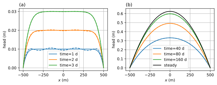
Figure 5.10 Transient infiltration between two rivers; early response with three terms (dashed) and ten terms (solid) (left) and late response with one term (dashed) and ten terms (solid) (right).

     At early times, the graph on the left shows that the head in the middle part of the aquifer rises at a rate \(N/S=0.01\) m/d, as discharge to the rivers does not have any draining effect on the middle part yet. When time progresses from 1 to 2 to 3 days, a larger and larger section of the aquifer drains toward the rivers. The head at \(t=160\) d approaches the steady state solution, as shown in the right graph.
     The characteristic time \(t_{95}\) of the system is defined here as the time it takes for the head to reach 95% of the steady state level. An approximate equation for \(t_{95}\) is obtained by first approximating the solution ((5.40)) with the first term in the series solution

(5.41)\[ h \approx \frac{-N}{2T}\left(x^2 - \tfrac{1}{4}L^2\right) - \frac{4NL^2}{\pi^3T} \cos\left[\frac{\pi x}{L}\right] \text{e}^{-t/\tau} \]

where

(5.42)\[ \tau = \frac{SL^2}{\pi^2T} \]

The cosine term may be further simplified with the first two terms of its Taylor series (\(\cos(x)\approx 1 - x^2/2\))

(5.43)\[ -\frac{4NL^2}{\pi^3T} \cos\left[\frac{\pi x}{L}\right] \approx -\frac{4NL^2}{\pi^3T}\left(1 - \frac{\pi^2x^2}{2L^2}\right) \approx \frac{N}{2T}\left(x^2 - \tfrac{1}{4}L^2\right) \]

where it is used that \(\tfrac{4}{2\pi}\approx \tfrac{1}{2}\) and \(\tfrac{8}{\pi^3}\approx \tfrac{1}{8}\). The head may now be approximated as

(5.44)\[ h \approx \frac{-N}{2T}\left(x^2 - \tfrac{1}{4}L^2\right)(1 - \text{e}^{-t/\tau}) \]

     It follows that at time \(t=\tau\), the head has reached \(1-\text{e}^{-1}=63\%\) of its final value, and at time \(t=3\tau\), the head has reached 95% of its final value. Hence, the characteristic time \(t_{95}\) may be approximated as

(5.45)\[ t_{95} \approx \frac{3SL^2}{\pi^2T} \]

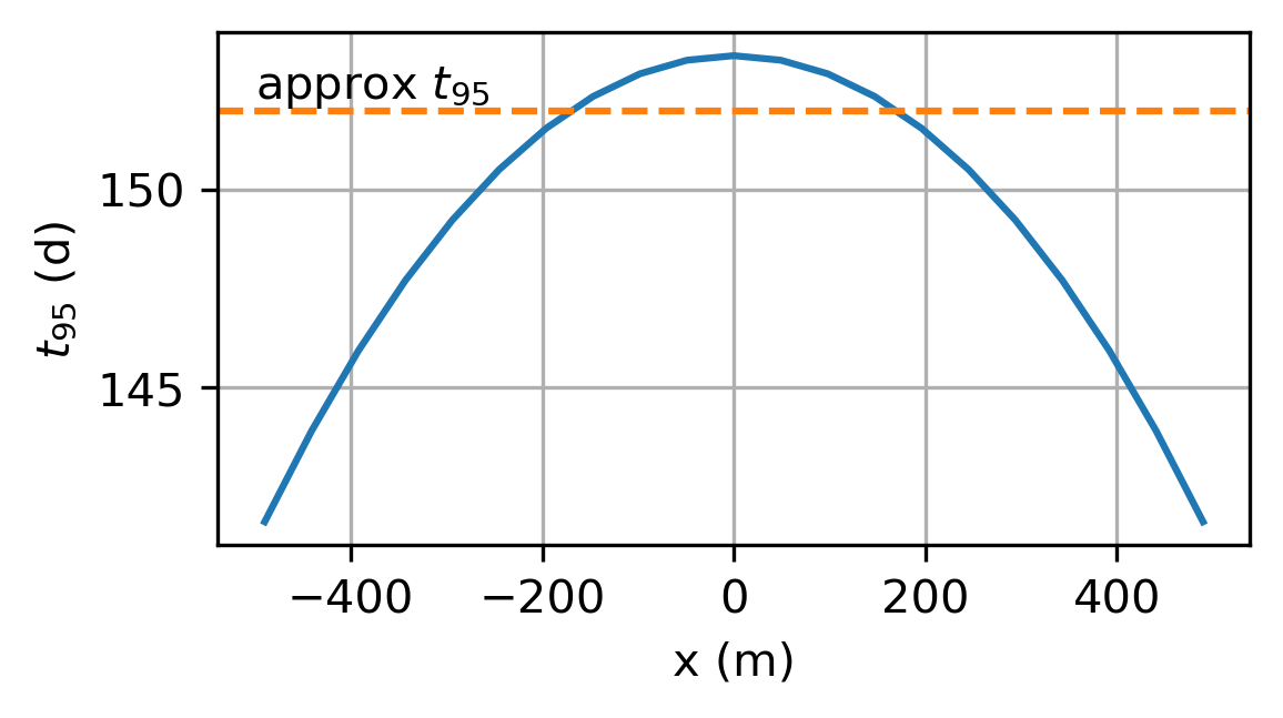
Equation ((5.45)) is a reasonable approximation of \(t_{95}\) for the entire aquifer, as is explored in the exercise below. The characteristic time \(t_{95}\) is also referred to as the memory of the system, as the head is back to its original value \(t_{95}\) after a recharge event ends. For the parameters used here, the value of \(t_{95}\) may be computed as

t95 = 3 * S * L**2 / (np.pi**2 * T)
print(f'The memory of the system is: {t95:0.0f} d')

The memory of the system is: 152 d

Exercise 5.6

Compute the memory of the system \(t_{95}\) using 10 terms in the solution for 20 equally spaced points between the two rivers, and plot the memory of the system vs. \(x\); use the fsolve method from scipy.optimize to find \(t_{95}\), similar to the use of fsolve in Section 3.2. In the same graph, plot \(t_{95}\) according to Eq. ((5.45)).

Solution

     Solution ((5.40)) is known as a step response: It is the response to a step in the recharge from zero to \(N\). The unit step response is the response to a unit step in the recharge from zero to one. In addition to the unit step response, there is the unit block response, which is the response to a unit of recharge per day for a period \(\Delta t\) and zero after that; \(\Delta t\) is referred to as the length of the block. The block response \(b\) is obtained through superposition of two step responses

(5.46)\[\begin{split} \begin{split} b(x, t) &= s(x, t) {\hskip 2em} 0 \le t \le \Delta t \\ b(x, t) &= s(x, t) - s(x, t-\Delta t) {\hskip 2em} t \ge \Delta t \end{split} \end{split}\]

where \(s(x,t)\)is the unit step response starting at \(t=0\), and \(s(x,t−\Delta t)\) is the unit step response starting at \(t=\Delta t\). The unit step response \(s(x,t)\) is computed with Eq. ((5.40)) by setting the recharge \(N\) to 1.
     The step response and block response are plotted at two locations in Figure 5.11. This represents the head response in an observation well at the specified value of \(x\). The block response is the same as the step response during the length of the block \(t\). The dotted lines in the corresponding colors represent the final steady levels of the step responses. The black dashed line indicates the head rise in the absence of the rivers (i.e., the head rise is \(N/S=0.01\) m/d). The head in the observation well farthest away from the rivers (in this case, at \(x=0\)) follows the dashed line for the longest period, up to ~20 days.
     The memory of the system is indicated with the vertical lines representing the \(t_{95}\) times for the step response and the block response; the latter is obtained as \(t_{95}\) after the block recharge has ended. Note that for this case, the memory of the system is 152 days, and the head in the aquifer is approximately back to its original value 152 days after the end of the recharge event.

# plot step recharge and response and block recharge and response at x=0
x = 0
delt = 365 / 12
t = np.linspace(0, 210, 211)
plt.subplot(221)
plt.plot([0, 210], [1, 1])
plt.subplot(222)
plt.plot([0, 30, 30, 210], [1, 1, 0, 0])
plt.subplot(223)
h = N * head(x, t, N=1)
plt.plot(t, h)
plt.subplot(224)
h[t > delt] -= N * head(x, t[t > delt] - delt, N=1)
plt.plot(t, h);

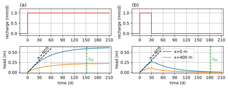
Figure 5.11 Step recharge (upper left) and the resulting step response with \(t_{95}\) after the start of step (lower left); block recharge for 30 days (upper right) and the resulting step response with \(t_{95}\) after the end of block (lower right); black dashed line is \(h=Nt/S\).

     The response to a series of recharge events of equal length \(\Delta t\) is computed using superposition. For example, if the recharge in the first three periods is \(N_0\), \(N_1\), and \(N_2\), then the head at \(t=0, \Delta t, 2\Delta t,\) and \(3\Delta t\) can be computed as

(5.47)\[\begin{split} \begin{split} &h|_{x,0} = 0 \\ &h|_{x,\Delta t} = N_0 b|_{x,\Delta t} \\ &h|_{x,2\Delta t} = N_0 b|_{x,2\Delta t} + N_1 b|_{x,\Delta t} \\ &h|_{x,3\Delta t} = N_0 b|_{x,3\Delta t} + N_1 b|_{x,2\Delta t} + N_2 b|_{x,\Delta t} \end{split} \end{split}\]

A Python implementation for three time steps is

N = np.array([1, 2, 3])
b = np.array([40, 20, 10])
h = np.zeros(4)
h[1] = np.sum(N[0] * b[0])
h[2] = np.sum(N[0] * b[1] + N[1] * b[0])
h[3] = np.sum(N[0] * b[2] + N[1] * b[1] + N[2] * b[0])
print(h)

[  0.  40. 100. 170.]

This can be generalized with a for loop, where it is used that b[n - 1::-1] stands for array b, starting at index n - 1 going to 0 with steps of -1 (i.e., backwards).

h = np.zeros(4)
for n in range(1, 4):
    h[n] = np.sum(N[:n] * b[n - 1::-1])
print(h)

[  0.  40. 100. 170.]

As an example, consider the following four years of recharge values (in mm/d) for monthly periods (the recharge is constant during each month). These recharge values are from an area with a temperate climate with a shallow water table and computed as the precipitation excess. The recharge is highest in the fall and winter, and can become negative in the spring and summer months when vegetation draws water from the water table.

# four years of monthly recharge data
delt = 365 / 12
recharge = 0.001 * np.array( # convert recharge from mm/d to m/d
[ 1.2,  1.5,  0.8, -1.2,  0.2, -2.9, -0.6,  2.8,  1.2,  0.9,  3.8,
  1.8,  1.9,  1.8, -0.6, -1.3, -2.5,  0.6,  0.9,  1.8, -0.3,  0.8,
 -0.2,  3.8,  2.8,  0.3, -0.5,  0.3, -1.1,  1.5,  1. , -1.5,  0.1,
  1.5,  1. ,  4. ,  1.3,  1.3,  0.3, -1.1,  0.6, -0.8, -1.2, -1.6,
  1.3,  1.4,  2.4,  2.6])
ntime = len(recharge) # number of month

     A function is written for the discrete block response \(b(x,n,\Delta t)\), which is the head response for a unit of recharge during a block of length \(\Delta t\). The discrete block response returns the head at ntime equal intervals \(\Delta t\).

# discrete block response
def bresponse(x, ntime, delt, T=T, S=S, L=L, nterms=10):
    t = np.linspace(delt, ntime * delt, ntime)
    return head(x, t, T, S, L, 1, nterms) - \
           head(x, t - delt, T, S, L, 1, nterms)

     The head is computed and plotted at two points in the aquifer through the outlined approach (Figure 5.12). Note that the unit block response is computed only once at each location. The yearly head variation halfway between the two rivers (\(x=0\)) is almost 2 m, while the head variation closer to the river is much smaller. The highest heads occur around January, and the lowest heads around July. The computed head in the first months (shown by a dashed line) is not very realistic as it is based on recharge since the beginning of the first year only, while the head also depends on the recharge in the previous year. After \(t_{95}=152\) days (the memory of this system), the effect of the previous year is negligible.

# solution
hl = np.zeros(ntime + 1) # head at x=0
h400 = np.zeros(ntime + 1) # head at x=400
b0 = bresponse(0, ntime, delt, T, S, L)
b400 = bresponse(400, ntime, delt, T, S, L)
for n in range(1, len(recharge) + 1):
    hl[n] = np.sum(recharge[0:n] * b0[n - 1::-1])
    h400[n] = np.sum(recharge[0:n] * b400[n - 1::-1])

# basic plot recharge data and head response
plt.subplot(211)
time = np.linspace(0, ntime * delt, ntime + 1)
plt.step(time[:-1], 1000 * recharge, where='post'); # plt.stairs in mpl>=3.4
plt.grid()
plt.subplot(212)
plt.plot(time, hl, label='$x=0$ m')
plt.plot(time, h400, label='$x=400$ m')
plt.legend();

Once Loop Reflect

Figure 5.12 Four years of monthly varying recharge (top) and the resulting transient head variation for recharge between two rivers; the head is dashed for part of series before \(t=t_{95}\).

     The head shown in Figure 5.12 is based on the exact solution ((5.40)). As a final example, it is investigated whether the head variation at \(x=0\) shown in Figure 5.12 can be simulated accurately with the simplified step response function

(5.48)\[ s(t)=A\left(1-\text{e}^{-t/a}\right) \]

The functional form of the simplified step response is the same as Eq. ((5.44)), but the parameters \(A\) and \(a\) are now simply fitting parameters. In other words, the head at \(x=0\) shown in Figure 5.12 is treated as the observed head in an observation well and the parameters \(A\) and \(a\) are obtained by performing a least squares fit. First, a function is written for the discrete block response corresponding to the simplified step response ((5.48)).

def simplebresponse(A, a, delt, nstep):
    t = np.linspace(0, nstep * delt, nstep + 1)
    hstep = A * (1 - np.exp(-t / a))
    return hstep[1:] - hstep[:-1]

     The difference \(\varepsilon\) between the observed head \(h_o\) and the modeled head \(h_m\), also called the residual or error, is computed as

(5.49)\[ \varepsilon = h_o - h_m \]

The optimal parameters \(A\) and \(a\) are found by minimizing the sum of squared errors, which is referred to as the objective function.

(5.50)\[ F_\text{obj} = \sum \varepsilon^2 \]

The first argument of the Python function for the objective function must be an array with the parameters. The final keyword argument is return_heads. When this keyword argument is set to True, the method returns the modeled heads rather than the sum of the squared errors, which is useful to compute the modeled heads after the parameters are estimated.

def fobj(p, delt=delt, recharge=recharge, hobs=hl, return_heads=False):
    A, a = p
    ntime = len(recharge)
    b = simplebresponse(A, a, delt, ntime + 1)
    hm = np.zeros(ntime + 1)
    for n in range(1, ntime + 1):
        hm[n] = np.sum(recharge[0:n] * b[n - 1::-1])
    if return_heads:
        return hm
    rv = np.sum((hobs - hm) ** 2)
    return rv

     The parameters that minimize the objective function may be found with a number of methods. Here, the fmin function of the scipy.optimize package is used, which applies the simplex algorithm (see the fmin documentation).

from scipy.optimize import fmin
A, a = fmin(fobj, [300, 20], disp=0)
print(f'Estimated parameters A: {A:.2f} d, a: {a:.2f} d')
print(f'Sum of the squared errors: {fobj([A, a]):.4f} m^2')
hm = fobj([A, a], return_heads=True) # compute modeled heads

Estimated parameters A: 629.89 d, a: 53.03 d
Sum of the squared errors: 0.0039 m^2

The modeled heads \(h_m\) fit the observed heads \(h_o\) very well (Figure 5.13).

# basic plot modeled heads
plt.plot(hl, 'C1.', label='observed')
plt.plot(hm, 'C0', label='modeled')
plt.legend();

The parameters \(A\) and \(a\) may be adjusted manually to try to fit the observed head in Figure 5.13.

Figure 5.13 Fit model with approximate response function to observations obtained with the exact solution for the response to four years of monthly varying recharge.

     The procedure discussed above, where a model of heads in an observation well is created with an approximate response function, is known as time series analysis. Time series analysis is a powerful and increasingly popular method to analyze heads measured in observation wells in fairly general settings. See, for example, Bakker and Schaars (2019) and Collenteur et al. (2019).

Exercise 5.7

Create a synthetic data set by computing 4 years of monthly heads at \(x=400\) m using the exact solution and the provided 4 years of monthly recharge. Apply time series analysis on the synthetic data set with the exponential response function ((5.48)). Report the fitted values of \(A\) and \(a\). Plot the modeled head and observed (synthetic) head in one graph.

Solution

\(A=218.85\) d, \(a=42.56\) d