7.3. A well in uniform background flow near a river

In many natural systems, groundwater flows towards a river in the absence of pumping. Pumping wells that are located near a river intercept the groundwater that is on its way to the river. Only when the discharge of a pumping well is large enough, part of the water pumped from the well will originate from the river. Either way, the flow in the river is depleted.
      In this section, wells are considered that are pumping near long and straight river sections, while the background flow is uniform and towards the river on both sides of the river. The aquifer is confined and has transmissivity \(T\). A well with discharge \(Q\) is located at \((x,y)=(-d,0)\) and the river runs along the \(y\)-axis. The river stage is \(h_R\), which corresponds to a potential \(\Phi_R=Th_R\). The river is in direct contact with the aquifer so the boundary condition along the \(y\)-axis is

(7.17)\[ \Phi|_{x=0,y}=\Phi_R \]

The background flow is uniform and normal to the river, but potentially different on either side of the river

(7.18)\[ Q_x = U_l {\hskip 2em} x \le 0 \]

(7.19)\[ Q_x = U_r {\hskip 2em} x \ge 0 \]

Note that because the river is in direct contact with the aquifer, the flow on the right side of the river remains uniform ((7.19)) even if there is a well on the left side. In Section 7.6, the bottom of the river is formed by a leaky stream bed.
     The discharge potential and stream function are obtained through the method of images and superposition as

(7.20)\[ \Phi = -U_l x + \frac{Q}{4\pi}\ln\frac{(x + d)^2 + y^2}{(x - d)^2 + y^2} + \Phi_r {\hskip 2em} x\le 0 \]

(7.21)\[ \Psi = -U_l y + \frac{Q}{2\pi}\left(\arctan\frac{y}{x+d} - \arctan\frac{y}{x-d}\right) {\hskip 2em} x\le 0 \]

The corresponding components of the discharge vector are

(7.22)\[\begin{split} Q_x = U_l - \frac{Q}{2\pi}\frac{x+d}{(x + d)^2 + y^2} + \frac{Q}{2\pi}\frac{x-d}{(x - d)^2 + y^2} {\hskip 2em} x\le 0 \\ \end{split}\]

(7.23)\[ Q_y = - \frac{Q}{2\pi}\frac{y}{(x + d)^2 + y^2} + \frac{Q}{2\pi}\frac{y}{(x - d)^2 + y^2} {\hskip 2em} x\le 0 \]

The critical discharge of the well is defined as the discharge at which the well doesn’t draw any water from the river into the aquifer. When the well pumps exactly at the critical discharge, the discharge vector at the point on the river closest to the well equals zero, so that the point \((x,y)=(0,0)\) is a stagnation point. An equation for the critical discharge \(Q_\text{cr}\) is obtained by setting \(Q_x\) (Eq. (7.22)) equal to zero at the origin, which gives

(7.24)\[ Q_\text{cr} = \pi U_l d \]

When the well pumps less than \(Q_\text{cr}\), the \(x\)-location of the stagnation point \(x_s\) is found by setting \(Q_x=0\) along \(y=0\), which gives

(7.25)\[ x_s = -\sqrt{d^2 - \frac{Qd}{\pi U_l}} {\hskip 2em} Q \le Q_{cr} \]

When the well pumps more than \(Q_\text{cr}\), there are two stagnation points along the river; water infiltrates from the river into the aquifer between these two stagnation points and flows towards the well. The locations \(y_s\) of the stagnation points along the river are found by setting \(Q_x=0\) along \(x=0\), which gives

(7.26)\[ y_s = \pm\sqrt{\frac{Qd}{\pi U_l} - d^2} {\hskip 2em} Q \ge Q_{cr} \]

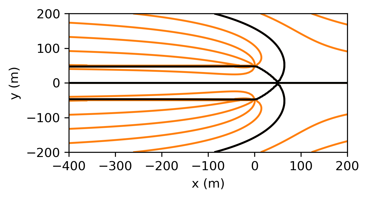
In the example below, the discharge of the well is larger than \(Q_{cr}\) (Figure 7.6). The flow net is shown on both sides of the river; flow is uniform on the right side of the river and not altered by the well (because the river is in direct contact with the aquifer and the Dupuit-Forchheimer approximation is adopted).
     In theory, the amount \(\Delta Q\) of the well discharge that originates from the river may be obtained by subtracting the values of the stream function at the stagnation points on the river. This is not possible here, because there is a branch cut between the well and the image well. Instead, the difference is taken between the stream function at the stagnation point and the stream function just on the positive side of the origin, which gives \(\tfrac{1}{2}\Delta Q\).

# parameters
dhdx = -0.001 # head gradient, -
hR = 10 # water level in river, m
T = 100 # transmissivity, m^2/d
Ul = -T * dhdx # uniform flow on left side of river, m^2/d
Ur = -Ul # uniform flow on right side of river, m^2/d
Q = 25 # discharge of well, m^3/d
d = 50 # distance between well and river, m
phiR = T * hR # potential along the river, m^3/d
Qcr = np.pi * Ul * d # critical discharge, m^3/d
print(f'Critial discharge {Qcr = :.2f} m^3/d')

Critial discharge Qcr = 15.71 m^3/d

# solution
def potential(x, y, Q, d=d, phiR=phiR):
    r1 = np.sqrt((x + d) ** 2 + y ** 2)
    r2 = np.sqrt((x - d) ** 2 + y ** 2)
    if x <= 0:
        pot = -Ul * x + Q / (2 * np.pi) * \
             np.log(r1 / r2) + phiR
    else:
        pot = -Ur * x + phiR
    return pot

def streamfunc(x, y, Q, d=d):
    theta1 = np.arctan2(y, x + d)
    theta2 = np.arctan2(y, x - d)
    if x <= 0:
        psi = -Ul * y + Q / (2 * np.pi) * (theta1 - theta2)
    else:
        psi = -Ur * y
    return psi

potvec = np.vectorize(potential) # vectorized version
psivec = np.vectorize(streamfunc)

xg, yg = np.meshgrid(np.linspace(-200, 50, 200), np.linspace(-100, 100, 200))
pot = potvec(xg, yg, Q)
psi = psivec(xg, yg, Q)
ys = np.sqrt(Q * d / (np.pi * Ul) - d ** 2) # positive y-location of stagnation point
half_delQ = streamfunc(0, ys, Q) - streamfunc(0, 1e-6, Q)
print(f'fraction of water from river for Q={Q} m^3/d: {2 * half_delQ / (Q):.2f}')

fraction of water from river for Q=25 m^3/d: 0.11

# basic flow nets
plt.subplot(111, aspect=1)
plt.contour(xg, yg, pot, np.arange(phiR - Q, phiR + Q, Q / 20))
plt.contour(xg, yg, psi, np.arange(-2 * Q, 3 * Q, Q / 20))

Figure 7.6 Flow net for a well in uniform background flow near a river with zero bed resistance, with \(Q_{cr} = 15.71\) m\(^3\)/d. Capture zone envelopes are shown in black. Discharge between two streamlines is \(\Delta\Psi=2\) m\(^3\)/d.

Exercise 7.6

For the parameters of the example above, compute the discharge of the well such that 25% of the well water originates from the river (you need a small Python script to do this).

Solution

\(Q=39.0\) m\(^3\)/d

Exercise 7.7

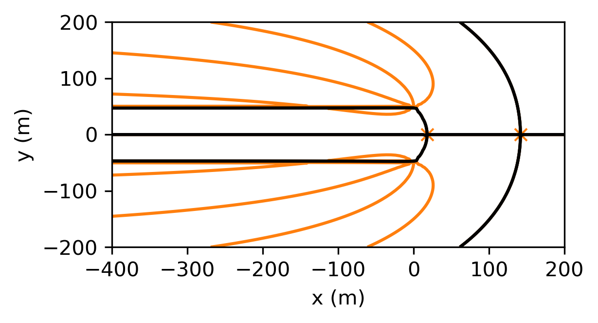
Consider two extraction wells with equal discharge \(Q\). One well is located at \((x,y)=(0, -50)\) and the other well at \((x,y)=(0, 50)\). The two wells are located in an otherwise uniform flow from West to East; the gradient far away is \(\partial h/\partial x=-0.002\). The transmissivity of the aquifer is \(T= 200\) m\(^2\)/d. Compute the minimum discharge \(Q_\text{min}\) so that no part of the background uniform flow passes between the two wells. Note that there are two stagnation points on the \(x\)-axis when \(Q>Q_\text{min}\). Draw the capture zone envelopes for two cases: \(Q=Q_\text{min}\) and \(Q=200\) m\(^3\)/d.

Solution

\(Q=125.7\) m\(^3\)/d