6.5. Wells in a two-aquifer system

In the previous section, the problem was solved for a well that pumps from the bottom aquifer of a two-aquifer system where the head in the top aquifer is constant and fixed. Here, a solution is presented for flow to a well in a two-aquifer systems where water flows in both aquifers. The well is screened in the bottom aquifer. The aquifers are numbered 0 and 1 from the top (see Figure 6.14). The transmissivities of the top and bottom aquifers are \(T_0\) and \(T_1\), respectively, and the resistance of the leaky layer between the aquifers is \(c\).

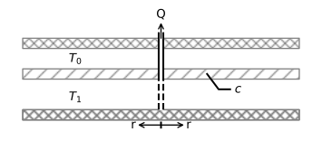
Figure 6.14 A well pumping in the bottom aquifer of a two-aquifer system.

      The flow in the two-aquifer system is governed by a system of two coupled differential equations (see Section 2.4)

(6.63)\[ \begin{align}\begin{aligned} &\nabla^2 h_0 = \frac{h_0-h_1}{cT_0}\\&\nabla^2 h_1 = \frac{h_1-h_0}{cT_1} \end{aligned}\end{align} \]

where \(h_0\) and \(h_1\) are the heads in the top and bottom aquifers, respectively. A well is pumping with a discharge \(Q\) in aquifer 1

(6.64)\[ \lim_{r \to 0} -2\pi r Q_{r,1} = Q \]

The second boundary condition is that the head is fixed to \(h_R\) at \(r=R\) in aquifer 0

(6.65)\[ h_0|_{r=R}=h_R \]

The solution for the head in each aquifer is a combination of the solution for a well in a confined aquifer (Eq. (6.37)) and the solution for a well in a semi-confined aquifer (Eq. (6.56))

(6.66)\[ \begin{align}\begin{aligned} & h_0 = \frac{Q}{2\pi(T_0+T_1)}\left[\ln(r/R)+\text{K}_0(r/\lambda) - \text{K}_0(R/\lambda)\right] + h_R\\& h_1 = \frac{Q}{2\pi(T_0+T_1)}\left[ \ln(r/R)+\frac{T_0\text{K}_0(r/\lambda)}{T_1} - \text{K}_0(R/\lambda)\right] + h_R \end{aligned}\end{align} \]

where

(6.67)\[ \lambda = \sqrt{ \frac{cT_0T_1}{T_0+T_1} } \]

The corresponding radial components of the discharge vector are

(6.68)\[ \begin{align}\begin{aligned} & Q_{r,0} = -\frac{T_0Q}{2\pi(T_0+T_1)} \left[ \frac{1}{r} - \frac{\text{K}_1(r/\lambda)}{\lambda}\right]\\& Q_{r,1} = -\frac{T_1Q}{2\pi(T_0+T_1)} \left[ \frac{1}{r} + \frac{T_0\text{K}_1(r/\lambda)}{T_1\lambda}\right] \end{aligned}\end{align} \]

Near the well, all flow is in aquifer 1, as can be seen from taking the limit and using that \(K_1(r/\lambda)\approx \lambda/r\) for small \(r\)

(6.69)\[ \begin{align}\begin{aligned} & \lim_{r\to 0} 2\pi r Q_{r,0} = 0\\& \lim_{r\to 0} 2\pi r Q_{r,1} = Q \end{aligned}\end{align} \]

Far away from the well (in practice, beyond \(4\lambda\)), the flow is distributed between the two aquifers according to their transmissivities

(6.70)\[ \begin{align}\begin{aligned} & \lim_{r\to \infty} 2\pi r Q_{r,0} = -\frac{T_0}{T_0+T_1}Q\\& \lim_{r\to \infty} 2\pi r Q_{r,1} = -\frac{T_1}{T_0+T_1}Q \end{aligned}\end{align} \]

In the example below, the head and total flow are plotted as a function of the radial distance (Figure 6.15). The head in the bottom aquifer shows a sharp drawdown at the well (\(r=0\)), while the head gradient equals zero at the well location in the top aquifer. The graph of the flow represents the total flow \(Q_\text{tot}=-2\pi r Q_r\) in the aquifer as a function of the radial distance. The sum of the total flow in the two aquifers always equals \(Q\). At the well, all flow is in the bottom aquifer, while far away from the well, the flow is distributed according to the transmissivities, as explained above. A streamline plot is shown for a cross section through the well in Figure 6.16.

# parameters
T0 = 100 # transmissivity aquifer 0, m^2/d
T1 = 150 # transmissivity aquifer 1, m^2/d
c = 1000 # resistance of leaky layer, d
zaq = [0, -10, -15, -25] # elevation of top of layers and bottom, m
R = 200 # distance where head is fixed, m
hR = 5 # head at r=R, m
Q = 1000 # discharge of well, m^3/d
rw = 0.3 # radius of well, m
lab = np.sqrt(c * T0 * T1 / (T0 + T1)) # leakage factor, m

# solution
from scipy.special import k0, k1
r = np.linspace(rw, 5 * lab, 200)
h0 = Q / (2 * np.pi * (T0 + T1)) * (np.log(r / R) + \
     k0(r / lab) - k0(R / lab)) + hR
h1 = Q / (2 * np.pi * (T0 + T1)) * (np.log(r / R) + \
     T0 * k0(r / lab) / T1 - k0(R / lab)) + hR
Q0tot = -Q * T0 / (2 * np.pi * (T0 + T1)) * (1 / r -
         k1(r / lab) / lab) * 2 * np.pi * r
Q1tot = -Q * T1 / (2 * np.pi * (T0 + T1)) * (1 / r + 
         T0 * k1(r / lab) / (T1 * lab)) * 2 * np.pi * r
psi = np.zeros((len(zaq), len(r)))
psi[1] = Q0tot
psi[2] = Q0tot
psi[3] = Q1tot + Q0tot

# basic plot head and flow
plt.subplot(121)
plt.plot(r / lab, h0, label='aquifer 0')
plt.plot(r / lab, h1, label='aquifer 1')
plt.legend()
plt.subplot(122)
plt.plot(r / lab, -Q0tot / Q, label='aquifer 0')
plt.plot(r / lab, -Q1tot / Q, label='aquifer 1')
plt.legend();

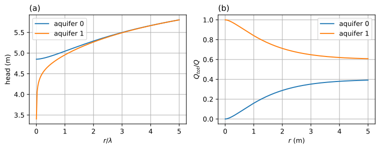
Figure 6.15 A well in the bottom aquifer of a two-aquifer system; head (left) and total flow (right).

# basic streamline plot for r >= 0
plt.contour(r, zaq, psi, 10);

Figure 6.16 Streamlines in a vertical cross section through a well (black dashed line) screened in the bottom aquifer of a two-aquifer system with \(\Delta\Psi=Q/10\).

Exercise 6.12

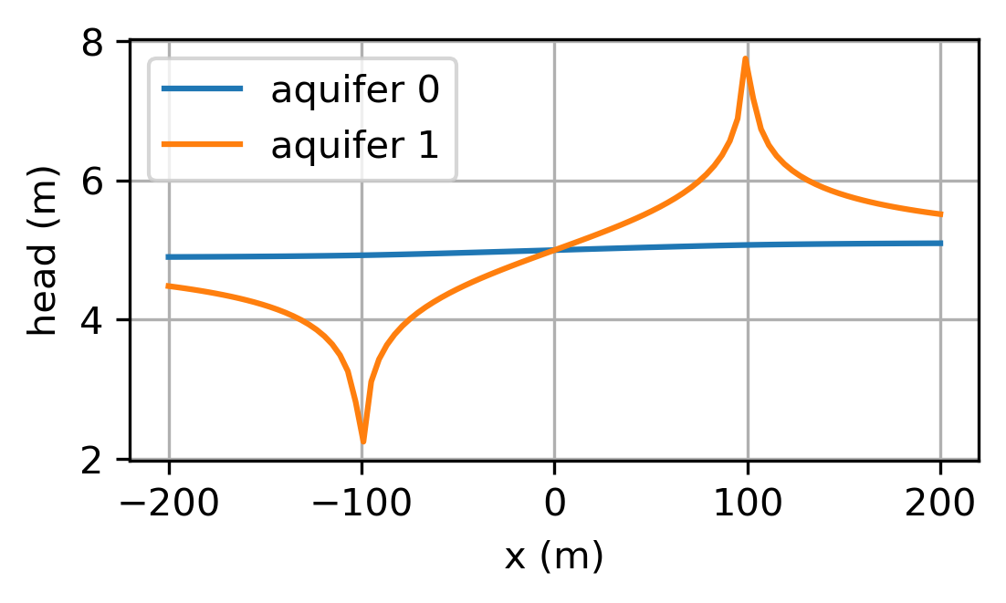
Consider an extraction well and an injection well pumping in the bottom aquifer. All parameters are as in the example. The extraction well is located at \((x,y)=(-100,0)\) and has a discharge \(Q=1000\) m\(^3\)/d, and the injection well is located at \((x,y)=(100,0)\) and has a discharge \(Q=-1000\) m\(^3\)/d; the radius of both wells is 0.3 m. The head far away from the doublet is 5 m. Plot the head along the line \(y = 0\), and compute the head at the extraction well in both aquifers.

Solution

\(h_0 = 4.93\) m
\(h_1 = 1.60\) m