2.3. Flow to a river of finite width

The next example considers one-dimensional steady flow to a long and straight river with width \(2L\). A vertical cross section normal to the river is shown in Figure 2.8. The origin of the coordinate system is chosen in the middle of the river. The flow is confined to the left and right of the river and semi-confined below the river. The resistance of the leaky river bed is \(c\), and the water level in the river is \(h^∗\). The transmissivity of the aquifer is \(T\). The flow is uniform and equal to \(Q_x=U_l\) in the aquifer to the left of the river, and the flow is uniform and equal to \(Q_x=U_r\) in the aquifer to the right of the river.

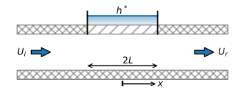
Figure 2.8 Flow to a long river of finite width.

      The head and flow below the river are solved first. Boundary conditions are

(2.27)\[ Q_x\vert_{x=-L}=U_l {\hskip 2em} Q_x\vert_{x=L}=U_r \]

The hyperbolic form (Eq. (2.9)) is used for the head solution below the river

(2.28)\[ h-h^* = A\sinh(x/\lambda) + B\cosh(x/\lambda) \]

with the corresponding solution for the discharge vector (Eq. (2.10))

(2.29)\[ Q_x=-\frac{AT}{\lambda}\cosh(x/\lambda) - \frac{BT}{\lambda}\sinh(x/\lambda) \]

      Substitution of the boundary conditions (Eq. (2.27)) in Eq. ((2.29)) gives

(2.30)\[ A = \frac{-\lambda(U_l + U_r)}{2T\cosh(L/\lambda)} {\hskip 2em} B = \frac{\lambda(U_l - U_r)}{2T\sinh(L/\lambda)} \]

The solutions for the head to the left and to the right of the river are simple linear functions, because the aquifer is confined. The solution below the river is used to compute the head \(h_0=h|_{x=-L}\) in the aquifer at the left river bank and the head \(h_1=h|_{x=L}\) in the aquifer at the right river bank. Once \(h_0\) and \(h_1\) are known, the solutions in the confined parts of the aquifer to the left and right of the river can be written as

(2.31)\[ h = -\frac{U_l}{T}(x + L) + h_0 {\hskip 2em} x\le -L \]

(2.32)\[ h = -\frac{U_r}{T}(x - L) + h_1 {\hskip 2em} x\ge L \]

An example is shown for the case that the width of the river is twice the leakage factor and the inflow at the left river bank is twice the inflow at the right river bank (Figure 2.9).

# parameters
k = 5 # hydraulic conductivity, m/d
H = 10 # aquifer thickness, m
hstar = 10 # head in river 
L = 100 # half width of river
c = 200 # resistance of leaky river bed, d
Ul = 0.1 # Qx in left aquifer
Ur = -0.05 # Qx in right aquifer
T = k * H # transmissivity, m^2/d
lab = np.sqrt(T * c) # leakage factor of aquifer below river
print(f'leakage factor: {lab:.0f} m')

leakage factor: 100 m

x = np.linspace(-300, 300, 100)
A = -lab * (Ul + Ur) / (2 * T) / np.cosh(L / lab)
B =  lab * (Ul - Ur) / (2 * T) / np.sinh(L / lab)
h0 = A * np.sinh(-L / lab) + B * np.cosh(-L / lab) + hstar
h1 = A * np.sinh(L / lab) + B * np.cosh(L / lab) + hstar
h = np.zeros(len(x))
h[x <= -L] = -Ul / T * (x[x <= -L] + L) + h0
h[x >= L]  = -Ur / T * (x[x >= L] - L) + h1
h[np.abs(x) < L] = A * np.sinh(x[np.abs(x) < L] / lab) + \
                   B * np.cosh(x[np.abs(x) < L] / lab) + hstar
Qx = np.zeros(len(x))
Qx[x <= 0] = Ul
Qx[x >= L] = Ur
Qx[np.abs(x) < L] = -A * T / lab * np.cosh(x[np.abs(x) < L] / lab) - \
                     B * T / lab * np.sinh(x[np.abs(x) < L] / lab)

# basic plot
plt.subplot(121)
plt.plot(x, h, 'C0')
plt.subplot(122)
plt.plot(x, Qx, 'C1');

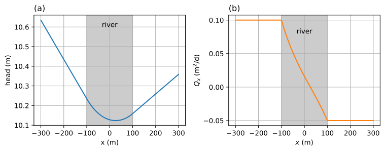
Figure 2.9 Groundwater flow to a river of finite width; head (left) and \(Q_x\) (right).

      Contours of the stream function are plotted below (Figure 2.10).

# solution
psi = np.zeros((2, len(x)))
psi[1] = -Qx
xg = x
zg = [0, H]

# basic streamline plot
plt.contour(xg, zg, psi, np.arange(-0.1, 0.05, 0.01));

Figure 2.10 Groundwater flow to a river of finite width; streamlines in a vertical cross-section. Discharge between two streamlines is \(\Delta\psi=0.01\) m\(^2\)/d.

Exercise 2.4

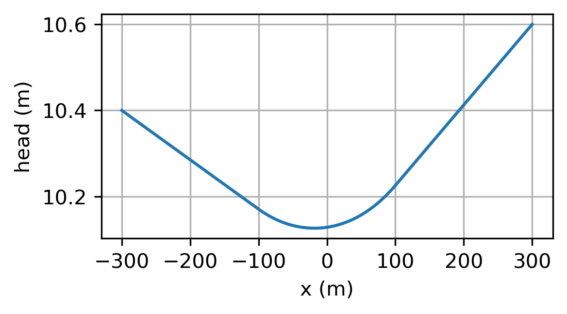
Consider the case that \(U_l\) and \(U_r\) are not known, but the head at \(x=-300\) m is measured to be 10.4 m, and the head at \(x=300\) m is measured to be 10.6 m. Solve for \(U_l\) and \(U_r\) using a root finding routine like scipy.optimize.fsolve. Plot the head as a function of \(x\).

Solution

\(U_l=0.0574\) m\(^2\)/d
\(U_r=-0.0936\) m\(^2\)/d