6.4. Wells in a semi-confined aquifer

Steady flow to a well in the bottom aquifer of a two-aquifer system is considered in the next two sections. The two aquifers are separated by a leaky layer. In this section, the head in the top aquifer is fixed, for example by a system of ditches and drains, so that the bottom aquifer is a semi-confined aquifer (Figure 6.12). The case for a two-aquifer system, where water is flowing through both aquifers, is presented in the next section. Recall that solutions for semi-confined flow and two-aquifer flow were written in terms of heads in Chapter 2 as the discharge potentials defined in Table (6.1) cannot be used.

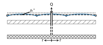
Figure 6.12 A well pumping in a semi-confined aquifer.

      The differential equation for steady radially symmetric semi-confined flow is

(6.53)\[ \nabla^2 h = \frac{\text{d}^2 h}{\text{d} r^2}+\frac{1}{r}\frac{\text{d} h}{\text{d}r} = \frac{h-h^*}{cT} \]

where \(T\) is the transmissivity of the aquifer, \(h^*\) is the constant head above the semi-confining layer, and \(c\) is the resistance to vertical flow of the semi-confining layer (see Chapter 2). A solution is sought for radial flow to a fully penetrating well with discharge \(Q\). The boundary condition at the well is the same as that for a well in confined flow

(6.54)\[ \lim_{r \to 0} -2\pi r Q_r = Q \]

The boundary condition at infinity is that the head is equal to the fixed head \(h^*\) in the top aquifer

(6.55)\[ h|_{r=\infty} = h^* \]

The solution is (De Glee, 1930)

(6.56)\[ h = h^* -\frac{Q}{2\pi T} \text{K}_0(r/\lambda) \]

where the leakage factor is \(\lambda=\sqrt{cT}\) (see Chapter 2) and \(\text{K}_0\) is the modified Bessel function of the second kind and order 0. The Bessel function \(\text{K}_0(r/\lambda)\) approaches zero for \(r\) approaching infinity. In practice, \(\text{K}_0\) can be approximated as zero for \(r>4\lambda\), as will be shown later.
      The main difference between the solutions for pumping in a confined aquifer and pumping in a semi-confined aquifer is that in a confined aquifer, all water pumped by the well comes from infinity (and hence the head keeps increasing toward infinity), while in a semi-confined aquifer, all water pumped by the well comes from the overlying aquifer by leakage through the semi-confining layer.
      The radial component of the discharge vector is obtained from differentiation

(6.57)\[ Q_r = -T\frac{\text{d}h}{\text{d}r} = \frac{-Q}{2\pi\lambda}\text{K}_1(r/\lambda) \]

where it is used that \(\text{dK}_0/\text{d}r = -\text{K}_1\), where \(\text{K}_1\) is the modified Bessel function of the second kind and order 1. It can be shown that \(Q_r\) fulfills boundary condition ((6.54)) by using that \(\text{K}_1\) may be approximated near \(r = 0\) as (e.g., Abramowitz and Stegun, 1965)

(6.58)\[ \text{K}_1 \approx \lambda / r {\hskip 2em} r/\lambda \ll 0 \]

The total flow \(Q_\text{tot}\) in the aquifer toward the well as a function of the radial distance \(r\) may be computed as \(-Q_r\) multiplied by the circumference of a circle with radius \(r\)

(6.59)\[ Q_\text{tot} = -2\pi r Q_r \]

Substitution of Eq. ((6.57)) for \(Q_r\) using Eq. ((6.58)) shows that boundary condition (Eq. (6.54)) is indeed fulfilled

(6.60)\[ Q_\text{tot} = -2\pi r \frac{-Q}{2\pi\lambda} \frac{\lambda}{r} = Q {\hskip 2em} r/\lambda \ll 0 \]

The head near the well may be approximated as

(6.61)\[ h = h^* + \frac{Q}{2\pi T} \ln\left(\frac{r}{1.123\lambda}\right) {\hskip 2em} (r/\lambda \ll 1) \]

where it is used that (Abramowitz and Stegun, 1965)

(6.62)\[ \text{K}_0(r/\lambda) \approx -\ln\left(\frac{r\text{e}^\gamma}{2\lambda}\right) \approx -\ln\left(\frac{r}{1.123\lambda}\right) {\hskip 2em} (r/\lambda \ll 1) \]

where \(\gamma=0.5772...\) is Euler’s constant. Note that Eq. ((6.61)) is the Thiem solution ((6.25)) where the head is equal to \(h^*\) at a distance of \(R=1.123\lambda\); the approximate formula gives accurate results near the well. The Bessel functions \(\text{K}_0\) and \(\text{K}_1\) are available as k0 and k1 in the scipy.special package.
      The solution for a well (Eq. (6.56)) and the approximate formula ((6.61)) near the well are plotted in the left graph of Figure 6.13. In the right graph, \(Q_\text{tot}\) is plotted as a function of \(r/\lambda\). Note that \(Q_\text{tot}/Q\) is indeed equal to 1 at the well and reduces to \(Q_\text{tot}/Q=0.05\) at \(r=4\lambda\). For practical purposes, the effect of the well may be neglected beyond a distance of \(4\lambda\).

# parameters
T = 200 # transmissivity of bottom aquifer, m^2/d
c = 1000 # resistance of leaky layer, d
hstar = 0 # fixed head in top aquifer, m
rw = 0.3 # radius of the well, m
lab = np.sqrt(T * c) # leakage factor, m
Q = 500 # discharge of well, m^3/d

# solution
from scipy.special import k0, k1
r = np.linspace(rw, 4 * lab, 200)
h = -Q / (2 * np.pi * T) * k0(r / lab) + hstar
happrox = Q / (2 * np.pi * T) * np.log(r / (1.123 * lab)) + hstar
Qtot = 2 * np.pi * r * Q / (2 * np.pi * lab) * k1(r / lab)

# basic plot
plt.subplot(121)
plt.plot(r / lab, h, label='head')
plt.plot(r / lab, happrox, label='approx')
plt.legend()
plt.subplot(122)
plt.plot(r / lab, Qtot / Q);

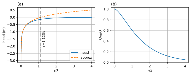
Figure 6.13 A well in a semi-confined aquifer; head (left) and total flow in the aquifer (right).

Exercise 6.10

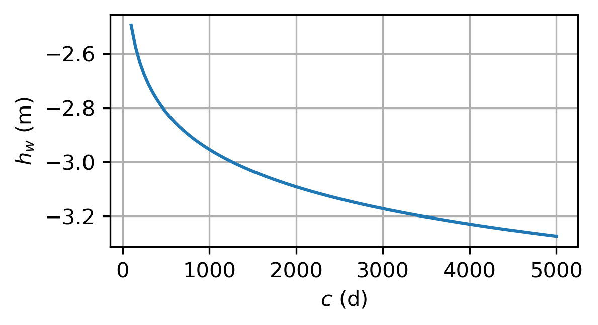
For the values of the example, compute the head at the well as a function of \(c\) for \(c\) varying from 100 d to 5000 d. Plot the head at the well vs. \(c\).

Solution

Exercise 6.11

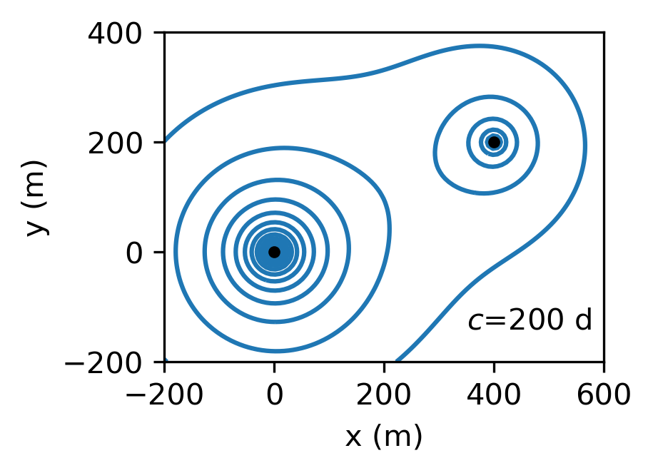
Consider two pumping wells in a semi-confined aquifer. Aquifer properties are \(T=200\) m\(^2\)/d, \(c=200\) d, \(h^*=-2\) m. Well 0 is located at \((x_0, y_0) = (0, 0)\) and has a discharge \(Q_0=500\) m\(^3\)/d, and well 1 is located at \((x_1, y_1)=(400, 200)\) and has a discharge \(Q_1=200\) m\(^3\)/d; the radius of the wells is 0.2 m. Make a contour plot of the heads in the aquifer. Compute the head at wells 0 and 1 for the case that \(c = 200\) d. Next, compute the head at wells 0 and 1 for the case that \(c = 1000\) d.

Solution

\(h_0 = -4.81\) m, \(h_1 = -3.15\) m for \(c = 200\) d
\(h_0 = -5.18\) m, \(h_1 = -3.41\) m for \(c = 1000\) d