5.5. Unconfined flow with variable transmissivity

So far in this chapter, the transmissivity of an aquifer has been approximated as constant, even when the flow was unconfined. This is a reasonable approximation when the variation of the saturated thickness is not too large, as was shown in Chapter 3 for steady unconfined flow. In this section, an alternative formulation for transient unconfined flow is presented and the accuracy of the constant transmissivity approximation is assessed.
     The one-dimensional continuity equation for transient unconfined flow is given by Eq. ((5.5)) as

(5.61)\[ \frac{\partial Q_x}{\partial x} = - S_p\frac{\partial h}{\partial t} + N \]

where \(S_p\) is the phreatic storage (or specific yield). \(Q_x\) may be written in terms of the discharge potential for unconfined flow as Eq. ((3.3))

(5.62)\[ Q_x = -\frac{\partial\Phi}{\partial x} \]

where \(\Phi\) is given by Eq. ((3.2))

(5.63)\[ \Phi = \tfrac{1}{2}k(h-z_b)^2 \]

where \(z_b\) is the elevation of the bottom of the aquifer. Substitution of Eq. ((5.62)) for \(Q_x\) in Eq. ((5.61)) gives

(5.64)\[ \frac{\partial^2 \Phi}{\partial x^2} = S \frac{\partial h}{\partial t} - N \]

This differential equation is known as the Boussinesq equation and is a nonlinear differential equation in terms of the head, because \(\Phi\) includes a term \(h^2\). This equation is notoriously difficult to solve analytically, even though it may not look all that complicated at first sight.
     The differential equation has to be linearized to solve it analytically. First, consider the derivative of \(\Phi\) (Eq. (5.63)) with respect to time

(5.65)\[ \frac{\partial \Phi}{\partial t} = k(h-z_b)\frac{\partial h}{\partial t} \]

Differential equation ((5.64)) may now be written as

(5.66)\[ \frac{\partial^2 \Phi}{\partial x^2} = \frac{S}{k(h - z_b)} \frac{\partial \Phi}{\partial t} - N \]

This equation is linearized by approximating the saturated thickness in front of the time derivative by a constant value \(\tilde{H}\)

(5.67)\[ \frac{\partial^2 \Phi}{\partial x^2} \approx \frac{S}{k\tilde{H}} \frac{\partial \Phi}{\partial t} - N \]

Differential equation ((5.67)) is a linear differential equation in terms of \(\Phi\). The solution for the discharge potential may be written as the sum of a steady solution and a transient solution.
     The problem of Section 5.1 is repeated, but now using the linearized Boussinesq equation for unconfined transient flow (Eq. (5.67)). A semi-infinite aquifer is bounded by a canal at \(x=0\). Initially, the head is equal to \(h_0\) so that the initial steady discharge potential equals

(5.68)\[ \Phi|_{x, t=0}= \Phi_0 =\tfrac{1}{2}k(h_0-z_b)^2 \]

At time \(t=0\), the head in the canal is raised by \(\Delta h\) (Figure 5.2) so that the discharge potential increases by an amount \(\Delta \Phi\)

(5.69)\[ \Delta \Phi = \tfrac{1}{2}k(h_0 + \Delta h -z_b)^2 - \Phi_0 \]

The boundary condition of the transient solution at \(x=0\) is

(5.70)\[ \Phi|_{x=0,t>0} = \Delta \Phi \]

while the head at infinity remains equal to \(h_0\)

(5.71)\[ \Phi|_{x\to\infty, t} = 0 \]

The transient solution for the discharge potential is (compare Eq. (5.14))

(5.72)\[ \Phi(x, t) = \Delta\Phi \, \text{erfc}(u) \]

where \(u\) is

(5.73)\[ u = \sqrt{\frac{S_px^2}{4k\tilde{H}t}} \]

The solution for the head is obtained from the total discharge potential (the steady solution plus the transient solution) in the regular way using Eq. ((3.7)) as

(5.74)\[ h = z_b + \sqrt{\Delta\Phi \, \text{erfc}(u) + \Phi_0} \]

     The example from Section 5.1 is resolved below. The linearized saturated thickness in the storage term is approximated as \(\tilde{H} = h_0 + \tfrac{1}{2}\Delta h\). The solution to the linearized Boussinesq equation is compared to the solution with constant transmissivity ((5.14)) of Section 5.1 using \(T=k\tilde{H}\) (Figure 5.16). For the numbers used in the example, the saturated thickness at \(x=0\) increases by 20%. The comparison shows only a small difference between the heads computed with the two methods, which means that the effect of a 20% increase in the saturated thickness is small. The difference in head computed with the two methods increases when the relative change in the saturated thickness is more dramatic, as is explored in the exercise below.

# parameters
k = 10 # hydraulic conductivity, m
zb = 0 # aquifer base, m
Sp = 0.2 # phreatic storage coefficient, -
h0 = 10 # initial head and canal level, m
delh = 2 # change in canal level, m
Ht = h0 + 0.5 * delh # linearized saturated thickness, m

from scipy.special import erfc
def h_unconfined(x, t, k, H, S, zb, h0, delh):
    pot0 = 0.5 * k * (h0 - zb) ** 2
    delpot = 0.5 * k * (h0 + delh - zb) ** 2 - pot0
    u = np.sqrt(S * x ** 2 / (4 * k * H * t))
    pot = delpot * erfc(u) + pot0
    return zb + np.sqrt(2 * pot / k)

# basic plot head
x = np.linspace(1e-12, 400, 100)
for t in [1, 10, 100]:
    h = h_edelman(x, t, k * Ht, Sp, delh) + h0 # from Section 5.1
    plt.plot(x, h)
    hun = h_unconfined(x, t, k, Ht, Sp, zb, h0, delh)
    plt.plot(x, hun)

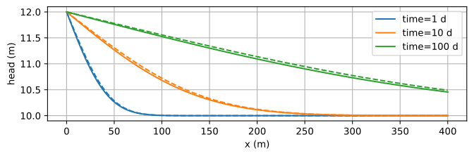
Figure 5.16 Head response to a change in the canal level at \(x=0\) using a constant transmissivity (solid lines) and a linearized saturated thickness in the storage term (dashed lines).

Exercise 5.9

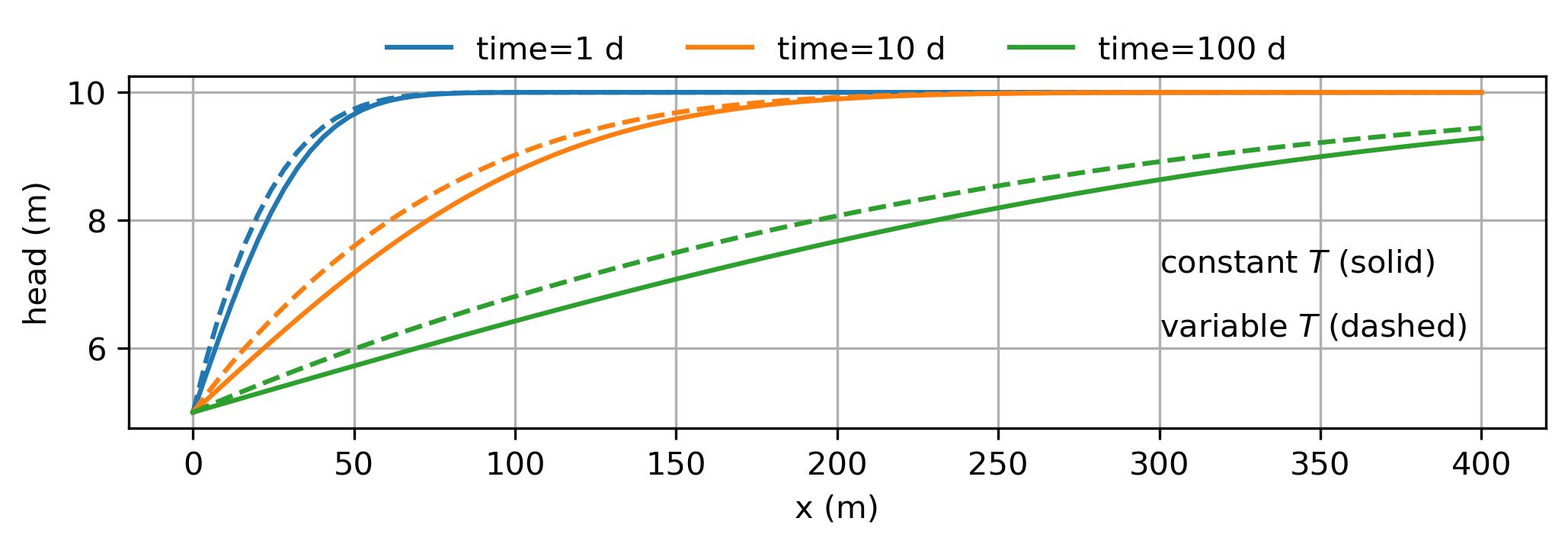
Compare the solution for unconfined transient flow presented here with the solution of Section 5.1 for the case that the head in the canal suddenly drops by 5 m. Compare the head in the aquifer after \(t=1, 10, 100\) days. Does this drastic (possibly unrealistic) change in the saturated thickness result in a significant difference between the two solutions?

Solution