6.1. Radially symmetric flow on a circular island

Radial flow problems and solutions are important in groundwater engineering because they represent the local flow field around pumping wells. In this section, solutions are presented for radially symmetric two-dimensional flow on a circular island. The head is fixed along the perimeter of the island, the areal recharge on the island is uniform, and a pumping well is located at the center of the island. The head and flow are a function only of the radial coordinate \(r\). The problem is depicted for unconfined flow in Figure 6.4, but is equally valid for any of the flow types listed in Table 6.1. The solution is derived as follows. First, the solution is derived for flow to a well at the center of a circular island without recharge (\(N = 0\)). Second, the solution is derived for flow on a circular island with uniform recharge, but no well (\(Q = 0\)). And third, the first two solutions are combined to solve the problem for flow to a well at the center of a circular island with uniform recharge. The purpose of this solution approach is to demonstrate the principle of superposition.
      The differential equation for the discharge potential in terms of r is given by Eq. ((6.8)). The general solution to this differential equation is

(6.20)\[ \Phi=-\frac{1}{4}Nr^2 +A\ln r + B \]

where \(A\) and \(B\) are constants to be evaluated from boundary conditions. The corresponding radial component of the discharge vector is

(6.21)\[ Q_r=-\frac{\text{d} \Phi}{\text{d}r} = \frac{1}{2}Nr - \frac{A}{r} \]

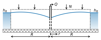
Figure 6.4 Unconfined flow to a well at the center of a circular island with radius \(R\) and uniform recharge.

First, consider flow to a pumping well at the center of a circular island of radius \(R\); the radius of the well is \(r_w\). The discharge potential that is the solution for this problem is referred to as \(\Phi_1\). The head is fixed to \(h_R\) at the perimeter of the island (\(r = R\)). The corresponding discharge potential is computed with the appropriate equation from Table 6.1 and is referred to as \(\Phi_R\)

(6.22)\[ \Phi_{1}|_{r=R}=\Phi_R \]

The discharge of the well is \(Q\) [L\(^3\)/T] and is positive for extracting water from the aquifer. The discharge is equal to the total flow into the well, which is the product of the discharge vector \(Q_r\) (Eq. (6.21)) at the perimeter of the well and the circumference of the well, resulting in the boundary condition

(6.23)\[ Q=-2\pi r_w Q_{r_1}|_{r=r_w} \]

Note the minus sign, as \(Q_r\) is defined as positive in the positive \(r\) direction, and the discharge \(Q\) of the well is positive for pumping water out of the aquifer. A slightly simpler boundary condition is

(6.24)\[ Q=\lim_{r_w \to 0}-2\pi r_w Q_{r_1}|_{r=r_w} \]

This condition often produces accurate results as the radius of the well is commonly much smaller than the horizontal scale of the groundwater problem being considered. Note that for this special case of a well at the center of a circular island without areal recharge, Eq. ((6.23)) is valid for any \(r\), not just at \(r_w\).
      Application of boundary conditions ((6.22)) and ((6.24)) to general solution ((6.20)), using \(N = 0\), results in the solution for the discharge potential

(6.25)\[ \Phi_1=\frac{Q}{2\pi}\ln{(r/R)} + \Phi_R \]

This is the potential form of the well-known Thiem equation (Thiem, 1906). The corresponding radial component of the discharge vector is

(6.26)\[ Q_{r_1} = -\frac{\text{d}\Phi_1}{\text{d}r} = -\frac{Q}{2\pi}\frac{1}{r} \]

Note that \(Q\) has the dimensions of a discharge (e.g., m\(^3\)/d), while \(Q_r\) is the radial component of the discharge vector with dimensions of discharge per unit length (e.g., m\(^2\)/d).
      Neither the discharge potential (and thus the head), nor the discharge vector can be calculated at the well, where \(r = 0\). In mathematical terms, such a point is called a singularity. The discharge potential (Eq. (6.25)), the corresponding head, and the discharge vector (Eq. (6.26)) have no physical meaning at the center of the well. These equations were derived for flow in the aquifer, but the aquifer stops at the well screen. Inside the well, the head is equal to the head in the aquifer just outside the well screen, provided the resistance to flow of the well screen is negligible. The head inside the well is computed by evaluating the head at the radius of the well (\(r = r_w\)).
      Next, consider uniform recharge on the island and no pumping well; this solution is referred to as \(\Phi_2\). As in the previous solution, the head (and thus the potential) is fixed at the perimeter of the island

(6.27)\[ \Phi_2|_{r=R}=\Phi_R \]

The second boundary condition is obtained from symmetry: The gradient of the head is zero at the center of the island, and hence, the flow is zero

(6.28)\[ Q_{r_2}|_{r=0}=0 \]

Application of these boundary conditions to the general solution ((6.20)) results in

(6.29)\[ \Phi_2 = -\frac{1}{4}N (r^2-R^2) + \Phi_R \]

The total amount of groundwater flow in the aquifer at the perimeter of the island is equal to the total recharge on the island, as is to be expected from continuity of flow

(6.30)\[ 2 \pi R Q_{r_2}|_{r=R} = N \pi R^2 \]

The flow at the perimeter is outflow, which is opposite to the first solution, in which flow at the perimeter is inflow.
      Finally, consider both a pumping well with discharge \(Q\) at the center of the island and uniform recharge \(N\) on the island. This problem contains both features of the first two solutions: recharge and a pumping well. The solution is referred to as \(\Phi_3\). The boundary conditions are

(6.31)\[ \Phi_3|_{r=R}=\Phi_R \]

and

(6.32)\[ \lim_{r_w \to 0}-2\pi r_w Q_{r_3}|_{r=r_w}=Q \]

Application of the boundary conditions to the general solution yields the following discharge potential

(6.33)\[ \Phi_3 = -\frac{1}{4}N (r^2-R^2) + \frac{Q}{2\pi} \ln{(r/R)} +\Phi_R \]

and the corresponding discharge vector

(6.34)\[ Q_{r_3} = \frac{Nr}{2} - \frac{Q}{2\pi}\frac{1}{r} \]

Comparison of the three solutions \(\Phi_1\), \(\Phi_2\), and \(\Phi_3\) (Eqs. (6.25), (6.29), and (6.33)) reveals that the third solution is the sum of the first two solutions except for the additive constant. Addition of multiple solutions to obtain another solution is an example of the principle of superposition, which is applicable to all linear differential equations, including the equations of Laplace and Poisson. The sum of the potentials of the first two problems satisfies the differential equation of the third problem

(6.35)\[ \nabla^2\Phi_3=\nabla^2(\Phi_1+\Phi_2)=\nabla^2\Phi_1+\nabla^2\Phi_2= 0 - N=-N \]

Similarly, the boundary condition at the well is satisfied by the sum of the two potentials. Finally, the value of the sum of the two potentials at \(r = R\) is a constant

(6.36)\[ \Phi_3|_{r=R}=\Phi_1|_{r=R}+\Phi_2|_{r=R}=2\Phi_R \]

This is not the value specified in the boundary condition (\(\Phi|_{r=R}=\Phi_R\)), but this is easily corrected by modification of the additive constant. In this example of superposition, two radially symmetric solutions were added such that the resulting solution is also two-dimensional radially symmetric flow, because the radial symmetry is about the same point (the center of the island).
      The flow rate and direction at the island’s perimeter depend on the relative magnitudes of the well discharge and the total recharge on the island. As an example, the head is computed for the case of unconfined flow in the code below. Two solutions are shown: the case for which the well pumps half the total areal recharge on the island and the case for which the well pumps exactly all the areal recharge on the island (Figure 6.5).

# parameters
k = 5 # hydraulic conductivity, m/d
zb = 0 # bottom elevation of aquifer, m
N = 0.001 # areal recharge, m/d
R = 200 # radius of the island, m
hR = 10  # head at edge of island, m
rw = 0.3 # well radius, m
Qhalf = 0.5 * N * np.pi * R ** 2  # discharge is half total recharge, m^3/d
Qtotal = N * np.pi * R ** 2  # discharge equals total recharge, m^3/d

# solution
r = np.linspace(rw, R, 400)
PhiR = 0.5 * k * (hR - zb) ** 2
Phi2 = -0.25 * N * (r ** 2 - R ** 2) + PhiR
Phi3 = Phi2 + Qhalf / (2 * np.pi) * np.log(r / R)
hhalf = zb + np.sqrt(2 * Phi3 / k)
Phi3 = Phi2 + Qtotal / (2 * np.pi) * np.log(r / R)
htotal = zb + np.sqrt(2 * Phi3 / k)

# basic plot head for half total discharge
plt.plot(-r, hhalf, 'C0', label='Q = half total recharge')
plt.plot(r, hhalf, 'C0')
plt.xticks(np.arange(-200, 201, 50), np.abs(np.arange(-200, 201, 50)))
plt.legend();

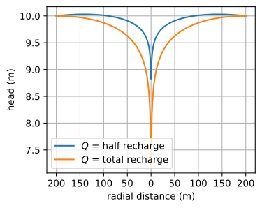
Figure 6.5 Head along centerline of a circular island for unconfined flow with uniform recharge and pumping well at the center of the island.

      As expected, the drawdown is much larger for the latter case than for the former case. Note that for the latter case, the flow at the perimeter of the island is zero and thus the slope of the water table is zero there. In the former case, there is still outflow across the island perimeter. Inflow occurs along the perimeter once the well discharge exceeds the total recharge on the island. The maximum discharge of the well is reached when the water level in the well (at \(r=r_w\)) is at the bottom of the aquifer.

Exercise 6.1

Consider the case of a well at the center of a circular island with recharge where the discharge of the well is equal to half the total recharge on the island, using the example values above. Compute the distance \(r_d\) from the center of the well to the water divide by setting \(Q_r|_{r=r_d}=0\). Compare the total recharge on a circle with radius \(r_d\) to the discharge of the well.

Solution

\(r_d = 141.4\) m

Exercise 6.2

Consider the case of a well at the center of a circular island with recharge where the discharge of the well is equal to half the total recharge on the island, using the example values above. Compute the total flow into the well at \(r=r_w\) by integrating \(Q_r\) around the well radius, and compare your answer to the discharge of the well. Is boundary condition ((6.24)) a good approximation?

Solution

\(Q = 62.83\) m\(^3\)/d

Exercise 6.3

For the example given above of a well at the center of a circular unconfined island with recharge, compute the maximum discharge of the well by setting the head at the well equal to the bottom of the aquifer.

Solution

\(Q = 251.2\) m\(^3\)/d