9.4. Wells with wellbore storage and skin effect

The previous solutions for transient flow to a well were based on two approximations: The boundary condition at the well was approximated by taking the limit for the well radius going to zero (Eq. (9.6)), and the water level in the well is approximated by the head at the well radius in the aquifer. The first approximation neglects the storage of the water inside the well, which is referred to as wellbore storage. The second approximation neglects the resistance of the well screen, which is referred to as the skin effect. Both are taken into account in this section.
      Consider radial flow to a well in a confined aquifer with transmissivity \(T\) and storage coefficient \(S\). The well starts pumping with discharge \(Q\) at time \(t = 0\). The radius of the well screen is \(r_w\) (see Figure 9.8). The resistance to flow through the well screen is equal to \(c_w\) so that the radial component of the discharge vector right at the well screen may be written as

(9.38)\[ Q_r|_{r=r_w} = H\frac{h_w - h|_{r=r_w}}{c_w} \]

where \(h_w\) is the water level inside the well. Conversely, the water level in the well may be written as

(9.39)\[ h_w = h|_{r=r_w} + \frac{c_w}{H}Q_r|_{r=r_w} \]

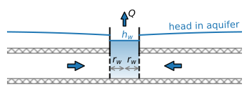
Figure 9.8 Vertical cross section through a well with wellbore storage and skin effect. The head in the aquifer at the well screen is higher than the water level \(h_w\) in the well because of the skin effect.

      The water balance for water inside the well is

(9.40)\[ A_w \frac{\text{d}h_w}{\text{d}t} = Q_\text{in} - Q_\text{out} \]

where \(A_w\) is the cross-sectional area of the well screen at the level of the water table in the well (\(A_w=\pi r_w^2\) for wells with a constant well radius). The inflow \(Q_\text{in}\) consists of the inflow integrated along the well screen

(9.41)\[ Q_\text{in} = -2\pi r_w Q_r|_{r=r_w} \]

while the outflow is equal to the discharge of the well

(9.42)\[ Q_\text{out} = Q {\hskip 2em} t\ge 0 \]

Substitution of Eq. ((9.39)) for \(h_w\), Eq. ((9.41)) for \(Q_\text{in}\), and Eq. ((9.42)) for \(Q_\text{out}\) in the water balance inside the well gives

(9.43)\[ A_w \left(\left.\frac{\partial h}{\partial t}\right|_{r=r_w} + \frac{c_w}{H} \left.\frac{\partial Q_r}{\partial t}\right|_{r=r_w}\right) = -2\pi r_w Q_{r}|_{r=r_w} - Q {\hskip 2em} t\ge 0 \]

      The governing differential equation for flow in the aquifer is the diffusion equation ((9.5)). The Laplace transform of the diffusion equation is the modified Helmholtz equation

(9.44)\[ \frac{\text{d}^2 \overline{h}}{\text{d} r^2}+\frac{1}{r}\frac{\text{d}\overline{h}}{\text{d}r}= \frac{Sp}{T}\overline{h}=w\overline{h} \]

where

(9.45)\[ w = Sp/T \]

The Laplace transform of the water balance inside the well (Eq. (9.43)) is

(9.46)\[ A_w p \overline{h}|_{r=r_w} + \left(\frac{A_w c_w p}{H} + 2\pi r_w\right) \overline{Q}_r|_{r=r_w} = - \frac{Q}{p} \]

      The general solution to the Laplace-transformed diffusion equation in radial coordinates (Eq. (9.44)), for the case that h equals zero far away, is

(9.47)\[ \overline{h}=B\text{K}_0(r\sqrt{w}) \]

where \(B\) is a parameter to be determined from the boundary conditions. The corresponding discharge vector in the Laplace domain is

(9.48)\[ \overline{Q}_r=-T\frac{\text{d}\overline{h}}{\text{d}r} = BT\sqrt{w}\text{K}_1(r\sqrt{w}) \]

Substitution of the equations for \(h\) and \(Q_r\) in the Laplace-transformed water balance (Eq. (9.46)) gives

(9.49)\[ B = -\frac{Q}{p} \frac{1}{A_w p \text{K}_0(r_w\sqrt{w}) + \left(\frac{A_w c_w p}{H} + 2\pi r_w\right) T \sqrt{w} \text{K}_1(r_w \sqrt{w}) } \]

Back-transformation of the Laplace-transformed solution to the time domain is again carried out using the Stehfest algorithm (see Section 5.4). Note that for the case that wellbore storage is neglected, the cross-sectional area \(A_w\) is set to zero in the water balance equation ((9.40)), which means that \((\pi r_w^2=0)\) and \(B\) reduces to

(9.50)\[ B = -\frac{Q}{p} \frac{1}{2\pi r_w T \sqrt{w} \text{K}_1(r_w \sqrt{w})} \]

which is the solution when the boundary condition at the well screen is

(9.51)\[ -2\pi r_w Q_r|_{r=r_w} = Q {\hskip 2em} t\ge 0 \]

In the example below, the head change is compared for a well without wellbore storage (boundary condition (9.51)), a well with wellbore storage but no skin effect, and a well with both wellbore storage and skin effect (Figure 9.9). For the values of the example, wellbore storage and skin effect have an effect on the head during the first few hours of pumping (\(t < 0.1\) d). For the case with skin effect, the head inside the well starts to differ from the head just outside the well after a few minutes of pumping (\(t > 0.002\) d).

# parameters
T = 200 # transmissivity, m^2/d
S = 0.005 # storage coefficient of aquifer, -
H = 10 # aquifer thickness, m
Q = 800 # discharge of well, m^3/d
rw = 0.3 # well radius, m
cw = 0.02 # resistance of well screen, d

# solution
from scipy.special import k0, k1
def hbar_wbs_res(p, r, T, S, Q, rw, cw, H): # hbar
    sqrtw = np.sqrt(S * p / T)
    Aw = np.pi * rw ** 2
    B = -Q / p * 1 / (p * Aw * k0(rw * sqrtw) + 
                     (2 * np.pi * rw + Aw * p * cw / H) * 
                      T * sqrtw * k1(rw * sqrtw))
    hbar = B * k0(r * sqrtw)
    return hbar

def Qrbar_wbs_res(p, r, T, S, Q, rw, cw, H): # Qrbar
    sqrtw = np.sqrt(S * p / T)
    Aw = np.pi * rw ** 2
    B = -Q / p * 1 / (p * Aw * k0(rw * sqrtw) + 
                     (2 * np.pi * rw + Aw * p * cw / H) * 
                      T * sqrtw * k1(rw * sqrtw))
    Qrbar = T * sqrtw * B * k1(r * sqrtw)
    return Qrbar

def hwbar_wbs_res(p, r, T, S, Q, rw, cw, H): # hbar inside well
    # r is not used, but Stehfest routine requires it
    hrw = hbar_wbs_res(p, rw, T, S, Q, rw, cw, H)
    Qrw = Qrbar_wbs_res(p, rw, T, S, Q, rw, cw, H)
    return cw * Qrw / H + hrw

# import stehfest_coef and stehfest from Section 5.4
t = np.logspace(-3, 0, 100)
ht = htheis(rw, t, T, S, Q) # function from Section 9.1
hw = stehfest(0, t, hwbar_wbs_res, T=T, S=S, Q=Q, rw=rw, cw=cw, H=H)
hwbs = stehfest(rw, t, hbar_wbs_res, T=T, S=S, Q=Q, rw=rw, cw=0, H=H)
hwbsres = stehfest(rw, t, hbar_wbs_res, T=T, S=S, Q=Q, rw=rw, cw=cw, H=H)

# plot of head at well
plt.semilogx(t, ht, label='x wbs, x skin')
plt.semilogx(t, hwbs[0], label=f'v wbs, x sin')
plt.semilogx(t, hwbsres[0], label=f'v wbs, v skin')
plt.semilogx(t, hw[0], '--', label=f'in well, v wbs, v skin')
plt.legend();

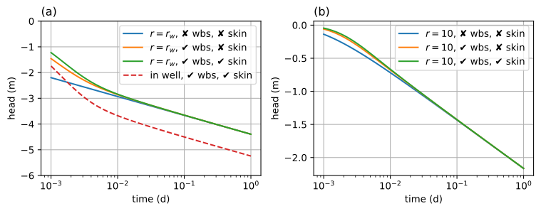
Figure 9.9 The effect of wellbore storage (wbs) and skin effect (skin) during the first day of pumping; head at the well (left) and head at \(r = 10\) m (right).

Exercise 9.9

Analyze the pumping test at Oude Korendijk (Section 9.1) taking into account wellbore storage using a well radius of 0.3 m, but no skin effect. Compare your answer to the results of Section 9.1.

Solution

Theis: \(T = 560\) m\(^2\)/d, \(S = 4.16 \cdot 10^{-5}\)