1.2. Areal recharge between two rivers

The transmissivity of an unconfined aquifer may be approximated as constant and equal to \(kH\) if the variation of the saturated thickness, caused by the change in water table elevation, is small compared to the total saturated thickness. In the following example, an unconfined aquifer is bounded on the left and right sides by two long parallel rivers that fully penetrate the aquifer (Figure 1.5). The rivers are a distance \(L\) apart and in direct contact with the aquifer so that

(1.20)\[ h\vert_{x=0} = h_l \]

(1.21)\[ h\vert_{x=L} = h_r \]

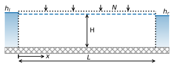
Figure 1.5 Areal recharge between two rivers.

      Because \(T\) is approximated as constant, the general equation ((1.8)) is still applicable and the integration constants for \(N > 0\) are

(1.22)\[ A=\frac{h_r-h_l}{L} + \frac{N}{2T}L \]

(1.23)\[ B=h_l \]

so that the solution becomes

(1.24)\[ h=-\frac{N}{2T}(x^2 - Lx) + \frac{(h_r-h_l)x}{L} + h_l \]

      The discharge vector \(Q_x\) is obtained by differentiation of Eq. ((1.24)) in combination with Eq. ((1.6))

(1.25)\[ Q_x = -T\frac{\text{d}h}{\text{d}x} = N\left(x - \frac{L}{2}\right) - T\frac{h_r-h_l}{L} \]

The solution is computed below. A slider is added to vary the head in the left river from \(h_l = 4\) m to \(h_l = 9\) m.

# parameters
L = 1000 # aquifer length, m
H = 10 # saturated thickness, m
zb = -5 # aquifer bottom, m
k = 10 # hydraulic conductivity, m/d
n = 0.3 # porosity, -
T = k * H # transmissivity, m^2/d
hl = 6 # specified head at the left boundary, m
hr = 4 # specified head at the right boundary, m
N = 0.001  # areal recharge, m/d

# solution
x = np.linspace(0, L, 100)
h = -N / (2 * T) * (x ** 2 - L * x) + (hr - hl) * x / L + hl
Qx = N * (x - L / 2) - T * (hr - hl) / L 

# basic plot
plt.subplot(121)
plt.plot(x, h)
plt.subplot(122)
plt.plot(x, Qx);

Figure 1.6 Areal recharge between two rivers; head (left) and \(Q_x\) (right).

      For the values given in the parameter block above, there is a groundwater divide between the two rivers (Figure 1.6). Part of the recharge flows to the left river, and part of the recharge flows to the right river. The discharge into the left river (\(x = 0\)) and the right river (\(x = L\)) are computed below. The flow into the left river plus the flow into the right river is exactly equal to the total recharge: \(NL = 1\) m\(^2\)/d. At the water divide, the head gradient equals zero so that \(Q_x = 0\).

print(f'discharge into left river: {-Qx[0]:.3f} m^2/d')
print(f'discharge into right river: {Qx[-1]:.3f} m^2/d')

discharge into left river: 0.300 m^2/d
discharge into right river: 0.700 m^2/d

Exercise 1.1

Compute the location of the water divide for the parameters that are provided above. Verify that the location of the water divide is consistent with the discharge figures computed above.

Solution

\(x_d = 300\) m

Exercise 1.2

Determine what the water level in the left river must be so that exactly all water that infiltrates flows to the right river, while no water from the left river flows to the right river; use the parameters of the example above. Plot \(h\) and \(Q_x\) vs. \(x\).

Solution

\(h_l = 9\) m

Exercise 1.3

Consider the case that \(h_l = h_r = 10\) m. The head halfway between the two rivers is measured to be 9 m. Compute the areal recharge for this case using the parameters of the example above. Plot \(h\) vs. \(x\).

Solution

\(N = -0.0008\) m/d

      In this solution, the flow is approximated as one-dimensional, and both \(h\) and \(Q_x\) are functions of \(x\) only. In a vertical cross section, however, the flow must be two-dimensional. After all, water infiltrates the aquifer at the top and discharges into the rivers to the left and right (see Figure 1.5). This leads to an apparent contradiction: How can water flow vertically in a one-dimensional solution?
      To resolve this contradiction, consider Darcy’s law for the vertical component of the specific discharge

(1.26)\[ q_z=-k_z \frac{\partial h}{\partial z} \]

where \(k_z\) is the hydraulic conductivity in the vertical direction. As the Dupuit–Forchheimer approximation is adopted, the head \(h\) is a function of \(x\) only, so \(\partial h/\partial z = 0\). This means that \(q_z\) is also equal to zero, except for the case that the vertical hydraulic conductivity \(k_z\) is infinitely large; the product of a term that goes to zero and a term that goes to infinity can result in a finite number (under certain mathematical conditions). Although this may seem strange at first (the vertical hydraulic conductivity is, of course, a finite number), this result can be interpreted to mean that the resistance to vertical flow is neglected (e.g., Strack, 1984). In other words, the energy it takes to flow vertically within an aquifer can be neglected with respect to the energy it takes to flow horizontally. This is often a good approximation, as groundwater commonly travels large distances horizontally (order of kilometers), but only small distances vertically (order of meters).
      The vertical component of the flow cannot be computed from Darcy’s law (as \(k_z = \infty\) causes all kinds of troubles), but can be obtained from continuity of flow. A differential equation for continuity of flow in the vertical \(x\), \(z\) plane may be derived by considering a vertical aquifer section that is \(\Delta x\) long and \(\Delta z\) high. The fluxes on the four sides are shown in Figure 1.7. Application of the volume balance for steady flow (In \(−\) Out = 0) gives

(1.27)\[ \left(\left.q_x\right|_{x+\Delta x, z} - \left.q_x\right|_{x, z}\right)\Delta z\Delta t+ \left(\left.q_z\right|_{x, z+\Delta z} - \left.q_z\right|_{x, z}\right)\Delta x\Delta t = 0 \]

Division by \(\Delta x \Delta z \Delta t\) and taking the limit for \(\Delta x\) and \(\Delta z\) going to zero gives

(1.28)\[ \frac{\partial q_x}{\partial x} + \frac{\partial q_z}{\partial z} = 0 \]

In mathematical terms, the divergence of the specific discharge vector equals zero for steady flow in the vertical plane.

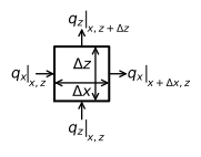
Figure 1.7 Two-dimensional continuity of flow in the vertical plane.

      The horizontal component \(q_x\) is obtained from the discharge vector (Eq. (1.25)) as

(1.29)\[ q_x= \frac{Q_x}{H} = -k\frac{\text{d}h}{\text{d}x} = \frac{N}{H}\left(x - \frac{L}{2} - \frac{T}{N}\frac{h_r-h_l}{L}\right) \]

Differentiation of \(q_x\) and substitution of the result in Eq. ((1.28)) gives

(1.30)\[ \frac{\partial q_z}{\partial z} = -\frac{N}{H} \]

which can be integrated to give

(1.31)\[ q_z=-\frac{Nz}{H} + C \]

The constant of integration \(C\) is obtained from the condition that at the impermeable base of the aquifer \((z=z_b)\), the vertical component of flow is zero so that \(C=Nz_b/H\) and

(1.32)\[ q_z=-\frac{N(z-z_b)}{H} \]

Note that the boundary condition at the top of the aquifer \(q_z\vert_{z=z_b + H}=-N\) is also satisfied, and that \(q_z\) decreases with depth according to a simple linear function. Expressions ((1.29)) and ((1.32)) are used below to create a streamplot for approximate two-dimensional flow in the vertical plane (Figure 1.8).

# solution
xg, zg = np.meshgrid(np.linspace(0, L, 10), np.linspace(zb, zb + H, 5))
qx = (N * (xg - L / 2) - T * (hr - hl) / L) / H
qz = - N * (zg - zb) / H

# basic stream plot
plt.subplot(111, aspect=25)
plt.streamplot(xg, zg, qx, qz, color='C1');

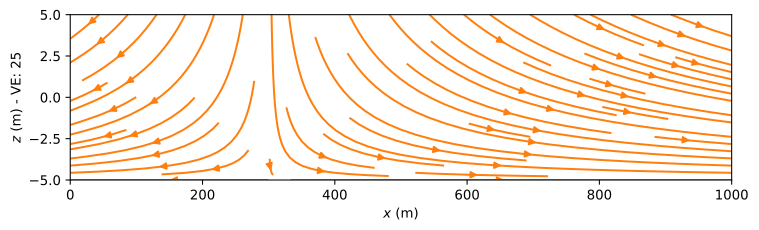
Figure 1.8 Streamplot in a vertical cross section for areal recharge between two rivers.

      A second method to visualize the two-dimensional flow field in a vertical cross section is to compute and contour the stream function. The stream function is a function that is constant along streamlines. The difference of the stream function values between two points is equal to the amount of water flowing between the two points, and the value of the stream function increases to the right when looking in the direction of flow.
      The stream function in a vertical cross section is denoted with the small Greek letter psi, \(\psi\) [L\(^2\)/T]. Here, \(\psi\) is arbitrarily set to zero along the impermeable base of the aquifer, as the impermeable base is a streamline. As a result, the stream function value along the top of the aquifer is equal to \(\psi = -Q_x\) so that the difference between the stream function values along the bottom and top of the aquifer is always equal to the discharge \(Q_x\) in the aquifer. The stream function value along the top of the aquifer is \(-Q_x\) and not \(Q_x\), because of the convention that the stream function increases to the right when looking in the direction of flow.
      A contour plot of the stream function is shown in Figure 1.9. It is created by defining an array psi of the stream function. The stream function is computed at a number of points along the bottom and top of the aquifer. The contouring routine interpolates linearly between the stream function computed along the top and bottom of the aquifer. This is exactly correct for this problem, as this means that the discharge is divided equally over the vertical. The amount of flow between two adjacent streamlines is always the same when a constant contouring interval is used (this is not the case for the lines obtained with the streamplot function used previously), so when two streamlines are closer together, water flows faster. In this case, the flow between two adjacent streamlines is \(NL/20\), as 20 contour intervals are plotted. The streamlines are evenly spaced every 50 m at the top of the aquifer, as the inflow is equal to \(q_z=-N\) there and \(L = 1000\) m. The vertical streamline that goes through the water divide is the dividing streamline and corresponds to a stream function value \(\psi=0\) (as this streamline continues along the bottom of the aquifer). The outflow to the right river is more than twice the outflow to the left river. Note that, indeed, the stream function increases to the right when looking in the direction of flow. The inflow along the top of the aquifer is uniform and equal to \(N\). The outflow into the rivers is also uniform in the vertical direction. This means, for example, that water that enters the aquifer halfway between the water divide and the river flows into the river at an elevation exactly equal to the middle of the aquifer.

# solution
x = np.linspace(0, L, 100)
Qx = N * (x - L / 2) - T * (hr - hl) / L 
psi = np.zeros((2, len(x)))
psi[1, :] = -Qx # at the top of the aquifer, the stream function is -Qx
xg = x
zg = [zb, zb + H]

# basic streamline plot
plt.subplot(111, aspect=25)
cs = plt.contour(xg, zg, psi, 20, colors='C1', linestyles='-')
plt.clabel(cs, fmt='%1.2f');

Figure 1.9 Streamlines in a vertical cross section for areal recharge between two rivers. Vertical exaggeration (VE) is 25. Discharge between two streamlines is \(\Delta\psi=0.05\) m\(^2\)/d.

      In the plot of the streamlines, the scales along the horizontal and vertical directions are not the same: The horizontal distance is actually 25 times larger than the vertical distance. When the scales along both axes are set equal, it is not possible to see the flow lines anymore for the entire cross section. For illustration purposes, the streamlines are plotted to scale (i.e., no vertical exaggeration) for the section from \(x = 500\) to \(x = 600\) in the figure below, showing that the streamlines are indeed predominantly horizontal (Figure 1.10).

# basic streamline plot of part of flow field without vertical exaggeration
plt.subplot(111, aspect=1, xlim=(500, 600))
cs = plt.contour(xg, zg, psi, 20, colors='C1', linestyles='-');

Figure 1.10 Streamlines in a vertical cross section for an area of the cross section shown in Figure 1.9 (no vertical exaggeration).

Exercise 1.4

Make a contour plot of the stream function for the case that the head in the left river is so high that exactly all water flows to the right river (i.e., the water divide is at the left river).

Solution

See Figure 1.9 with slider at \(h_l=9\) m.

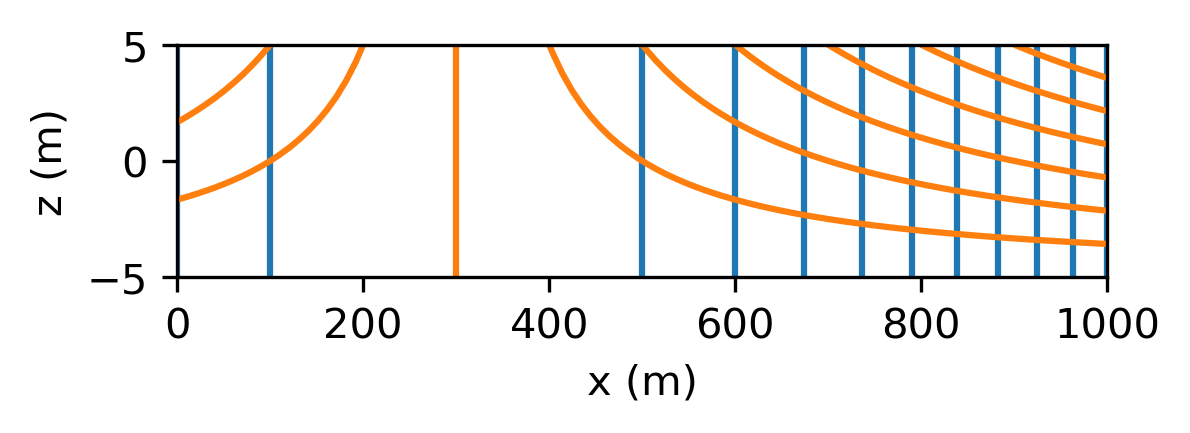
      It is common practice to draw contours of the head and streamlines on the same plot, as they form what is called a flow net where the streamlines cross the head contours at right angles, as will be demonstrated for two-dimensional solutions in later chapters. This is only the case when the hydraulic conductivity is isotropic. Here, the solution for flow in the vertical plane is based on the Dupuit–Forchheimer approximation, which is equivalent to the case where the vertical hydraulic conductivity is much larger than the horizontal hydraulic conductivity so that the head contours and streamlines don’t form a flow net.

Exercise 1.5

Draw a flow net showing head contours and streamlines for the example on the same graph.

Solution

      The travel time for water that enters at the top of the aquifer and leaves the aquifer at the left or right river can again be computed from the horizontal component of the velocity vector \(v_x=q_x/n\) (since \(v_x\) is not a function of the vertical coordinate), as was done in the previous section. This gives the travel time \(t_\text{tr}(x_0, x_1)\) from location \(x=x_0\) to location \(x=x_1\)

(1.33)\[ t_\text{tr}(x_0, x_1) = \int_{x_0}^{x_1} \frac{\text{d}x}{v_x} = \frac{nH}{N} \ln\left[\frac{v_x|_{x=x_1}}{ v_x|_{x=x_0}}\right] \]

Similarly, the travel time from the top of the aquifer \(z_b + H\) to elevation \(z\) is obtained from the vertical component of the velocity vector \(v_z=q_z/n\), which gives

(1.34)\[ t_\text{tr}(z) = \int_{z_b+H}^z \frac{\text{d}z}{v_z} = \frac{nH}{N}\ln\left(\frac{H}{z - z_b}\right) \]

The travel time from the top of the aquifer to elevation \(z\) is only a function of \(z\). That is an interesting result, famously obtained by Vogel (1967), because it means that all water at a certain depth has the same age for this case of uniform recharge.

Exercise 1.6

Compute how long it takes for water that enters the aquifer at the top of the aquifer halfway between the water divide and the right river to flow to the right river. Use the parameters of the example and a porosity \(n = 0.3\). Compute the travel time in two ways: using the equation for the travel time from \(x_0\) to \(x_1\), and the equation for the travel time from the top of the aquifer to halfway the thickness of the aquifer. They should, of course, give the same answer.

Solution

\(t_\text{tr} = 2079\) d