10.6. Interface flow below a strip island

Two-dimensional steady interface flow in the vertical plane is explored further by considering interface flow in a cross-section of a strip island; the saltwater is at rest. The distance between the two shores (i.e., the width of the island) is \(2L\), and the infiltration rate is equal to \(N\) (Figure 10.20). Flow is unconfined, but the small variation in the phreatic surface is neglected and the top of the aquifer is approximated as horizontal at the same elevation as the sea bottom. The origin of the coordinate system is chosen at the top of the aquifer in the center of the island. The sea bottom is horizontal and the head along the sea bottom is set equal to zero.

(10.58)\[ h\vert_{x>L,z=0} = h\vert_{x<-L,z=0} = 0 \]

The stream function along the interface is set equal to zero.

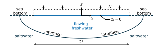
Figure 10.20 Two-dimensional interface flow in a vertical cross-section of a strip island.

      The complex specific discharge potential solution to the stated problem is obtained from Bruggeman (1999, Eq. 910.03), modified for the coordinate system chosen here. The solution has the following form

(10.59)\[ \omega^2 +2i N\zeta\omega + kN \zeta^2/\alpha - N(N + k/\alpha)L^2 = 0 \]

Note that Eq. ((10.59)) is a second-order polynomial in \(\omega\). A solution for \(\omega\) for a given value of \(\zeta\) is obtained using the standard formula for the root of a parabola, which gives

(10.60)\[ \omega = -iN\zeta + \sqrt{N^2(L^2 - \zeta^2) + Nk(L^2 - \zeta^2)/\alpha} \]

The specific discharge potential along the interface equals \(\phi_i=-kz_i\alpha\), so that an equation for the elevation of the interface as a function of \(x\) may be obtained by substituting \(\omega=-kz_i\alpha\) for \(\omega\) and \(x+iz_i\) for \(\zeta\) in Eq. ((10.59)), which gives (after considerable algebra)

(10.61)\[ z_i = -\sqrt{ \frac{N\alpha}{k}L^2 - \frac{N\alpha}{N\alpha+k} x^2} \]

The shape of the interface is an ellipse and the locations of the shorelines are the foci of the ellipse. The location \(x_\text{tip}\) of the tip of the interface is obtained by setting \(z_i=0\) in Eq. ((10.61)), which gives

(10.62)\[ x_\text{tip} = \pm L\sqrt{1 + \frac{N\alpha}{k}} \]

The elevation of the interface at the center of the island is obtained by setting \(x=0\) in Eq. ((10.61)), which gives

(10.63)\[ z_i|_{x=0} = -L\sqrt{\frac{N\alpha}{k}} \]

A flow net is constructed as follows. First, the location of the tip is computed with Eq. ((10.62)). Second, an array of \(x\) values is created from \(-x_\text{tip} + \varepsilon\) to \(-x_\text{tip} - \varepsilon\), where \(\varepsilon\) is a small number (\(\varepsilon\) is used to make sure that the first point is numerically not to the left of \(-x_\text{tip}\) and the last point is numerically not to the right of \(+x_\text{tip}\)). Third, a grid of \(z\) values is computed between the interface and the top of the aquifer for every \(x\)-value. Fourth and final, \(\omega\) is computed on the grid and a flow net is contoured.
      In the example below, the width of the island equals 2000 m; the flow net is shown in Figure 10.21. The freshwater zone is a bit more than 63 m thick at the center of the island, while the outflow zone is only 2 m on each side. Note that, contrary to other flow nets in this chapter, the vertical scale is exaggerated in Figure 10.21 (otherwise the figure would be unreadable), which makes the flow net resemble flow in an anisotropic aquifer while this is not the case.

# parameters
k = 10 # hydraulic conductivity, m/d
L = 1000 # half width of island, m
N = 0.001 # areal recharge, m/d
rhof = 1000 # density freshwater, kg/m^3
rhos = 1025 # density of saltwater, kg/m^3
alpha = rhof / (rhos - rhof)

# solution
def omega(zeta, k=k, alpha=alpha, L=L, N=N):
    om = -1j * N * zeta + np.sqrt(N ** 2 * (L ** 2 - zeta ** 2) + 
                                  N * k * (L ** 2 - zeta ** 2) / alpha)
    return om

# compute interface
ng = 201
xtip = L * np.sqrt(1 + N * alpha / k)
print(f'length outflow zone: {xtip - L:0.2f} m')
xi = np.linspace(-xtip + 1e-12, xtip - 1e-12, ng)
zi = -np.sqrt(N * alpha / k * L ** 2 - N * alpha / (N * alpha + k) * xi ** 2)
zcenter = -L * np.sqrt(N * alpha / k)
print(f'elevation of interface at center of island: {zcenter:0.2f} m')
# compute grid for contouring
xg = xi * np.ones((50, ng))
zg = np.zeros_like(xg)
for i in range(ng):
    zg[:, i] = np.linspace(zi[i], -1e-12, 50)
om = omega(xg + 1j * zg)

length outflow zone: 2.00 m
elevation of interface at center of island: -63.25 m

# basic plot
plt.subplot(111, aspect=5, xlim=(-xtip, xtip))
plt.contour(xg, zg, om.imag, 20)
plt.contour(xg, zg, om.real, 20)
plt.plot(xi, zi, 'k');

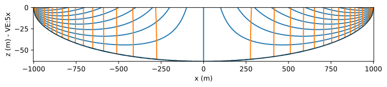
Figure 10.21 Flow net for two-dimensional interface flow in a cross-section of a strip island with isotropic hydraulic conductivity (note vertical exaggeration VE=5\(\times\)).

      The solution for an anisotropic hydraulic conductivity is obtained using the approach of Section 10.1. In addition, the infiltration rate \(\tilde{N}\) in the transformed domain is

(10.64)\[ \tilde{N}=N\sqrt{k_x/k_z} \]

The resulting equation for the elevation of the interface is

(10.65)\[ z_i = -\sqrt{ \frac{N\alpha}{k_x}L^2 - \frac{N\alpha}{N\alpha+k_z} \frac{k_z}{k_x}x^2} \]

Hence, the elevation of the interface at the center of the island is

(10.66)\[ z_i|_{x=0} = -\sqrt{ \frac{N\alpha}{k_x}L^2} \]

This result may be surprising, as it means that the depth of the interface at the center of the island only depends on the horizontal component \(k_x\) of the hydraulic conductivity and not on the vertical component. Conversely, the equation for the tip of the interface only depends on \(k_z\) and not on \(k_x\)

(10.67)\[ x_\text{tip} = L\sqrt{1 + \frac{N\alpha}{k_z}} \]

This means that the length of the outflow zone is larger when the vertical hydraulic conductivity is smaller.
      The solution for two-dimensional flow in the vertical plane is compared to the Dupuit solution. The Dupuit solution for the interface is obtained from Section 4.2 as

(10.68)\[ z_{i} = -\sqrt{\frac{N\alpha}{k_x}(L^2-x^2)} \]

so that the Dupuit elevation of the interface at the center of the island is

(10.69)\[ z_{i}|_{x=0} = -\sqrt{ \frac{N\alpha}{k_x}L^2} \]

which is exactly the same as the two-dimensional solution (Eq. (10.66)) irrespective of the vertical hydraulic conductivity! Everywhere else, the Dupuit solution is conservative: the thickness of the freshwater zone is smaller than in the two-dimensional solution.
      In the example below, the interface obtained with the Dupuit solution is compared to the two-dimensional solution for the case that the hydraulic conductivity is isotropic and for a case that the hydraulic conductivity is anisotropic. The Dupuit solution is again a very good and conservative approximation (Figure 10.22).

# additional parameters for anisotropic case
kx = k
kz = kx / 20

# solution
xtipaniso = L * np.sqrt(1 + N * alpha / kz)
xaniso = np.linspace(-xtipaniso + 1e-12, xtipaniso - 1e-12, 400)
zianiso = -np.sqrt(N * alpha / kx * L ** 2 - 
                   N * alpha / (N * alpha + kz) * kz / kx * xaniso ** 2)
xdupuit = np.linspace(-L, L, 200)
zidupuit = -np.sqrt(N * alpha / kx * (L ** 2 - xdupuit ** 2))

# basic plot
plt.subplot(111, aspect=5)
plt.plot(xi, zi, label='2D, $k_z=k_x$')
plt.plot(xdupuit, zidupuit, '--', label='Dupuit')
plt.plot(xaniso, zianiso, label='2D, $k_z=k_x/20$')
plt.legend();

Figure 10.22 Comparison of the interface position below a strip island for the anisotropic, two-dimensional solution and the Dupuit solution.

Exercise 10.8

Compute the ratio of the depth of the interface and the head at the interface at \(x=0\) for the anisotropic case. Next, compute ratio of the depth of the interface and the head at the top of the aquifer at \(x=0\) for the anisotropic case.

Solution

Factor based on the head at the interface at \(x=0\) m: \(40\)
Factor based on the head at the top of the aquifer at \(x=0\) m: \(38.5\)