5.4. Solutions with Laplace transforms

As mentioned, there are various mathematical approaches to obtain solutions for transient groundwater flow problems. One of these approaches is the Laplace transform, which was originally applied to derive, e.g., the solution in Section 5.1. In the Laplace transform method, the governing partial differential equation is transformed into an ordinary differential equation in what is called the Laplace domain. The solution to the ordinary differential equation in the Laplace domain is much easier than the solution to the original partial differential equation. The difficulty lies in the back-transformation from the Laplace domain to the time domain, which requires the solution of a complicated integral. Luckily, there are several algorithms to carry out the integration numerically when analytic integration is cumbersome or impossible. There are entire books written on Laplace transformations, including useful tables with transformations of mathematical functions. A nice introduction for the mathematically inclined groundwater engineer or hydrogeologist is given by Bruggeman (1999). Here, a very brief introduction is given by demonstrating how to solve the problem of Section 5.1 for the case that the initial head equals zero.
     The Laplace transform is an integral transform, indicated with the symbol \(\mathcal{L}\), and is defined as

(5.51)\[ \mathcal{L}\{h\} = \bar{h}(x,p) = \int_0^\infty h(x,t)\text{e}^{-pt}\text{d}t \]

where \(\bar{h}\) is the Laplace-transformed head, which is a function of \(x\) and the Laplace transform parameter \(p\), but not of time. The transforms of derivatives with respect to \(x\) are simple

(5.52)\[ \mathcal{L}\left\{ \frac{\partial h}{\partial x} \right\} = \frac{\partial \bar{h}}{\partial x} {\hskip 2em} \mathcal{L}\left\{ \frac{\partial^2 h}{\partial x^2} \right\} = \frac{\partial^2 \bar{h}}{\partial x^2} \]

while transformation of the derivative with respect to time is

(5.53)\[ \mathcal{L}\left\{ \frac{\partial h}{\partial t} \right\} = p \bar{h} \]

Application of the Laplace transformation rules to the governing differential equation (5.8) for transient one-dimensional flow without recharge gives

(5.54)\[ \frac{\text{d} ^2 \bar{h}}{\text{d} x^2} = \frac{pS}{T}\bar{h} \]

which is indeed an ordinary differential equation. Eq. ((5.54)) is the modified Helmholtz equation ((2.5)), which was introduced in Chapter 2 for steady semi-confined flow.

Boundary conditions need to be transformed as well. Transformations of all kinds of functions can be found in tables of Laplace transforms. The Laplace transform of the constant \(\Delta h\) gives

(5.55)\[ \mathcal{L}\{\Delta h\} = \int_0^\infty \Delta h \text{e}^{-pt}\text{d}t = \frac{\Delta h}{p} \]

     The solution to differential equation ((5.54)) with transformed boundary conditions results in an equation for \(\bar{h}(x,p)\); this solution is referred to as the Laplace domain solution. The ultimate interest is of course a function \(h(x,t)\), which is obtained through what is called the backtransformation or the inverse Laplace transformation. Several approaches exist to find the inverse transform (e.g., Bruggeman, 1999), but they are often difficult or even impossible to carry out analytically. This has spurred the development of several approximate algorithms to perform the back-transformation. The Stehfest algorithm is one of the most popular methods and is used here (Stehfest, 1970).
     The Stehfest approximation of the inverse transformation is a weighted mean of the solution in the Laplace domain for a number of values of the Laplace parameter \(p_k\) (\(k=1,...,M\)). Hence, the application of the Stehfest approximation requires evaluation of \(\bar{h}(x,p)\) for a number of values of the Laplace parameter \(p\) to compute the value of the head at location \(x\) and time \(t\). The number of terms in the approximation is \(M\), which must be even. The Stehfest formula is

(5.56)\[ h(x, t) = \frac{\ln 2}{t} \sum_{k=1}^M V_k \bar{h}(x, p_k) \]

where \(M\) is the number of terms, \(V_k\) is the weight for term \(k\), and \(p_k\) is the Laplace parameter \(k\) computed as

(5.57)\[ p_k = \frac{k\ln 2}{t} \]

In theory, the approximation is more accurate when more terms are used, but machine accuracy is quickly causing a problem. The summation in Eq. ((5.56)) consists of the summation of increasingly larger positive and negative numbers. For large values of the index \(k\) in the summation, these numbers are so large that they only differ beyond the 16\(^\text{th}\) digit. Python normally only keeps track of 16 digits, which means that the sum of a positive and negative number that only differ beyond the 16\(^\text{th}\) digit essentially results in garbage. Luckily, it is fairly obvious when too many terms are used, as the result is obviously wrong.
     The formula for the parameters \(V_k\) is rather lengthy

(5.58)\[ V_k = (-1)^{k+M/2} \sum_{j=\text{int}[(k+1)/2)]} ^ {\min(k,M/2)} \frac{j^{M/2}(2j)!} {(\tfrac{M}{2}-j)!j!(j-1)!(k-j)!(2j-k)!} \]

The formula for \(V_k\) is implemented in the routine below (adopted from the mpmath package by Johansson and others, 2013).

# coefficients V_k
from scipy.special import factorial as fac
def stehfest_coef(M):
    assert M % 2 == 0, 'M must be even' # make sure M is even
    M2 = int(M / 2)
    V = np.zeros(M)
    for k in range(1, M + 1):
        z = np.zeros(min(k, M2) + 1)
        for j in range(int((k + 1) / 2), min(k, M2) + 1):
            z[j] = j ** M2 * fac(2 * j) / \
            (fac(M2 - j) * fac(j) * fac(j - 1) * fac(k - j) * fac(2 * j - k))
        V[k - 1] = (-1) ** (k + M2) * np.sum(z)
    return V

     The Stehfest algorithm ((5.56)) is implemented in the routine below. The first two input arguments are the \(x\) locations and times \(t\) for which the function is computed. Both input arguments x and t may be arrays. The next input argument is a Python implementation of the Laplace-transformed function that can be called as func(p, x, keyword_arguments), where keyword_arguments can be an arbitrary number of keyword arguments. The next input argument is the keyword argument \(M=12\), which is the default number of terms used in the Stehfest algorithm. Finally, an arbitrary number of keyword arguments may be supplied. These keyword arguments are passed to the function func of the Laplace-transformed solution (the keyword_arguments mentioned above). The stehfest function returns a two-dimensional array with shape (len(x), len(t)). Note that the parameters \(V_k\) are only a function of \(M\), so they are computed only once. The Laplace parameters \(p_k\) must be computed separately for each time with Eq. ((5.57)).

# Stehfest algorithm
def stehfest(x, t, func, M=12, **kwargs):
    t = np.atleast_1d(t)
    x = np.atleast_1d(x)
    f = np.zeros((len(x), len(t)))
    V = stehfest_coef(M)
    for i in range(len(t)):
        p = np.arange(1, M + 1) * np.log(2) / t[i]
        for j in range(len(x)):
            fbar = func(p, x[j], **kwargs)
            f[j, i] = np.log(2) / t[i] * np.sum(V * fbar)
    return f

     In the code blocks that follow, the transient problem of Section 5.1 (the groundwater response to a change \(\Delta h\) in the river stage in a semi-infinite confined aquifer) is re-solved using Laplace transforms. The differential equation in the Laplace domain is ((5.54)), and the boundary conditions are

(5.59)\[\begin{split} \begin{split} &\bar{h}\vert_{x=0}=\frac{\Delta h}{p} \\ &\bar{h}\vert_{x\to\infty}=0 \end{split} \end{split}\]

Mathematically, this is the same as the problem solved in Section 2.1. The solution is

(5.60)\[ \bar{h} = \frac{\Delta h}{p} \exp(-x\sqrt{pS/T}) \]

The solution in the time domain is obtained with the Stehfest algorithm, and the Stehfest solution is compared to the exact solution.

# parameters
T = 100 # transmissivity, m^2/d
S = 0.2 # storage coefficient, -
delh = 2 # increase in river level, m

# Laplace-transformed solution
def hbar(p, x, T=100, S=1e-3, delh=2):
    return delh / p * np.exp(-x * np.sqrt(p * S / T))

# comparison
x = 50 # location, m
t = 10 # time, d
M = 12 # number of terms
V = stehfest_coef(M)
hx = h_edelman(x, t, T, S, delh=2) # from Section 5.1
hs = stehfest(x, t, hbar, M=M, T=T, S=S)
print(f'Exact head at x={x} m and t={t} d: {hx}')
print(f'Stehfest head with M={M} terms  : {hs}')
print(f'Relative error: {(hs - hx) / hx}')

Exact head at x=50 m and t=10 d: 1.2341501549039475
Stehfest head with M=12 terms  : [[1.23415675]]
Relative error: [[5.34718718e-06]]

     The relative error is on the order of \(10^{−6}\) with \(M=12\) terms in the Stehfest solution. The relative error is plotted versus the number of Stehfest terms in Figure 5.14. Note that the relative error starts to increase again when more than 20 terms are used; this many terms should be avoided.

Mlist = np.arange(2, 33, 2)
error = np.zeros(len(Mlist))
for i, M in enumerate(Mlist):
    hs = stehfest(x, t, hbar, M=M, T=T, S=S)
    error[i] = np.abs((hs - hx) / hx)

# simple plot
plt.semilogy(Mlist, error, '-', marker='.')
plt.xticks(np.arange(2, 33, 2));

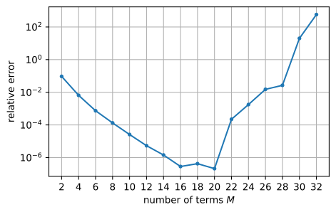
Figure 5.14 Relative error of the Stehfest solution as a function of the number of terms \(M\) used in the Stehfest algorithm.

     The lowest relative error is on the order of \(10^{−6}\). This means that the Stehfest algorithm can be expected to be accurate to up to about six significant digits. The head is computed and plotted vs. \(x\) at three different times (Figure 5.15). The error is shown in the right graph of Figure 5.15.

# solution
x = np.linspace(1e-12, 200, 100)
t = [1, 10, 100]
hx = np.empty((len(x), 3))
for itime in range(3):
    hx[:, itime] = h_edelman(x, t[itime], T, S, delh) # h_edelman from Sec. 2.1
hs = stehfest(x, t, hbar, M=12, T=T, S=S)

# basic plot head and error
plt.subplot(121)
plt.plot(x, hs)
plt.subplot(122)
plt.plot(x, hs - hx);

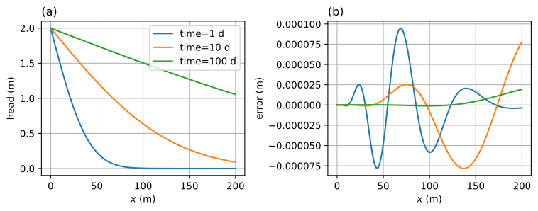
Figure 5.15 Stehfest solution for transient flow caused by a change in river stage; head (left) and Stehfest solution minus Edelman solution (right).

Exercise 5.8

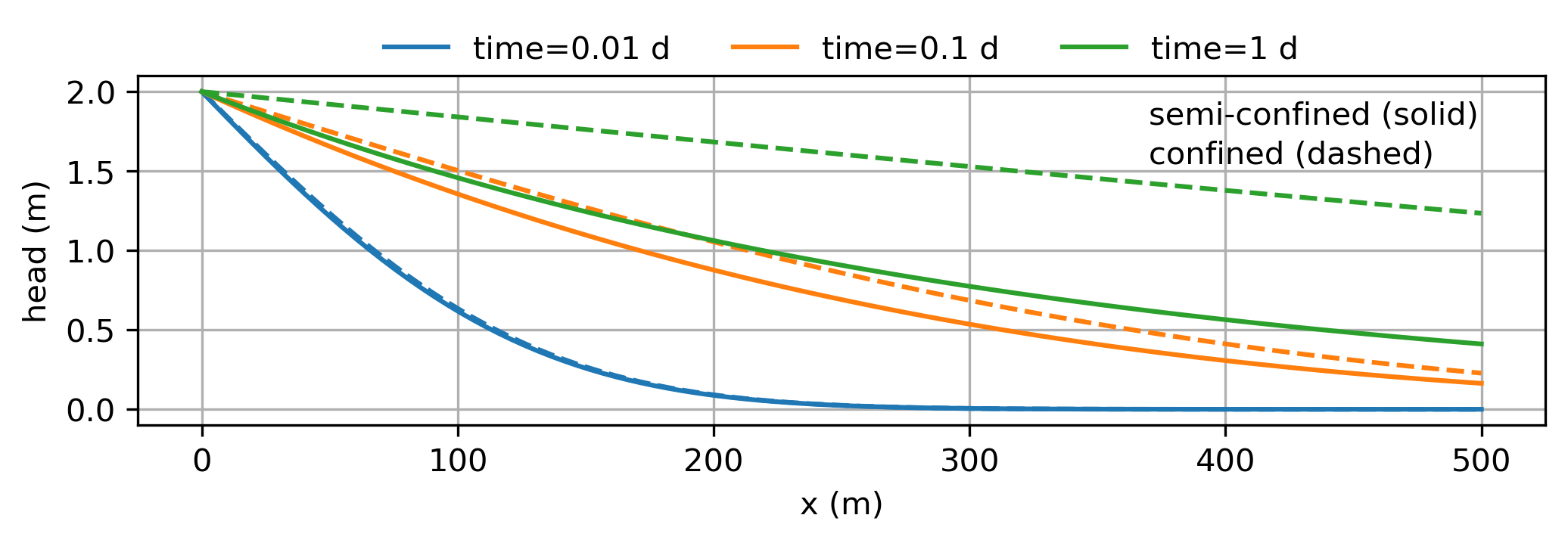
Solve the transient flow problem of Section 5.1 with the Laplace transform method, but for the case that the aquifer is semi-confined. Use \(T=100\) m\(^2\)/d, \(S=2\cdot 10^{-4}\), and \(c=1000\) d for the resistance of the leaky layer. Reproduce the left graph of Figure 5.15 for \(x\) varying from 0 till 500 and \(t=0.01\), \(0.1\), and \(1\) day; plot the solution for both the confined and semi-confined cases in the same graph. Report the head at \(x=100\) m at \(t=0.01\), \(0.1\), and \(1\) day.

Solution

\(h=0.618\) m at \(t=0.01\) d
\(h=1.356\) m at \(t=0.1\) d
\(h=1.458\) m at \(t=1\) d