7.6. A well in uniform background flow near a river with a leaky stream bed

The solution for a well in a uniform background flow near a long and straight river segment in direct contact with the aquifer of Section 7.3 is modified to include a leaky streambed below the river. The solution is obtained with the complex potential. All boundary conditions are the same as for the solution in Section 7.3, except for the boundary condition along the river. The river has a leaky streambed so that there is a hydraulic resistance between the river and the aquifer (Figure 7.10). Therefore, the pumping well on one side of the river results in a drawdown on the other side of the river, unlike in Section 7.3. The pumping well may capture water from the other side of the river, which can have major implications for a safe groundwater supply, e.g., when there is a contamination on the other side of the river (Harr, 1962) .
      The river has a small width \(B\) and the streambed has a resistance to vertical flow \(c\). Leakage to or from the river is approximated as occurring along the centerline of the stream and the width of the stream is neglected in the solution. This approximation may be reasonable when the stream is narrow relative to the aquifer thickness and the leakage factor (\(\sqrt{kHc}\)). The vertical specific discharge through the leaky streambed is written as

(7.41)\[ q_z = \frac{h - h_R}{c} \]

The inflow \(\sigma\) [L\(^2\)/T] from the aquifer into the river per unit length of river is obtained as

(7.42)\[ \sigma(y) = Bq_z = B\frac{h|_{x=0,y} - h_R}{c} = \frac{C}{T}(\Phi|_{x=0,y} - \Phi_R) \]

where the conductance of the streambed is defined as \(C = B/c\). The boundary condition along the river is obtained from continuity of flow as

(7.43)\[ \sigma = Q_x|_{x=0^-,y} - Q_x|_{x=0^+,y} = \frac{C}{T}(\Phi|_{x=0,y} - \Phi_R) \]

where \(x=0^-\) and \(x=0^+\) are the \(x\)-locations just to the left and right of the center line of the river, respectively. The second boundary condition along the river is that the head in the aquifer on the left side of the river is equal to the head in the aquifer on the right side of the river, or in terms of the discharge potential (recall that the width \(B\) of the river is neglected in the solution)

(7.44)\[ \Phi|_{x=0^-,y} = \Phi|_{x=0^+,y} \]

The uniform background flow on both sides of the river is the same as ((7.18)) and ((7.19)) (see also Figure 7.6).

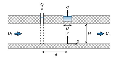
Figure 7.10 Vertical cross-section of well near river with leaky stream bed.

      The complex potential solution to the stated problem is obtained from Bakker and Anderson (2003). The complex potential is

(7.45)\[ \Omega = \frac{Q}{2\pi} \ln\frac{\zeta+d}{d-\zeta} - \frac{Q}{2\pi}\exp(Z_0)\text{E}_1(Z_0) - U_l\zeta + A {\hskip 2em} x \le 0 \]

(7.46)\[ \Omega = -\frac{Q}{2\pi}\exp(Z_1)\text{E}_1(Z_1) - U_r \zeta + A {\hskip 2em} x \ge 0 \]

where

(7.47)\[ Z_0 = -\frac{C}{2T}(\zeta-d) \]

(7.48)\[ Z_1 = \frac{C}{2T}(\zeta+d) \]

(7.49)\[ A = \frac{T}{C}(U_l-U_r) + \Phi_R \]

and \(\text{E}_1\) is the exponential integral, which is available as exp1 in the scipy.special package of special functions. The corresponding complex discharge vector is

(7.50)\[ W = -\frac{Q}{2\pi} \left[ \frac{1}{\zeta + d} + \frac{C}{2T}\exp(Z_0)\text{E}_1(Z_0)\right] + U_l {\hskip 2em} x \le 0 \]

(7.51)\[ W = -\frac{Q}{2\pi} \left[ \frac{1}{\zeta + d} - \frac{C}{2T}\exp(Z_1)\text{E}_1(Z_1)\right] + U_r {\hskip 2em} x \ge 0 \]

The complex potential is implemented in the following function

# parameters
T = 100 # transmissivity, m^2/d
hR = 10 # water level in river, m
Ul = 0.1 # uniform flow on left side of river, m^2/d
Ur = -0.1 # unform flow on right side of river, m^2/d
d = 50 # distance between well and river, m
phiR = T * hR # potential along the river, m^3/d
rw = 0.3 # radius of well, m
kstreambed = 0.02 # hydraulic conductivity of streambed, m/d
Hstreambed = 0.2 # thickness of streambed, m
B = 5 # width of streambed, m
c = Hstreambed / kstreambed #  resistance of stream bed, d
C = B / c # conductance of streambed, m/d
print(f'leakage factor below stream: {np.sqrt(T * c):.0f} m')

leakage factor below stream: 32 m

# solution
from scipy.special import exp1

def omegaresriv(x, y, Q):
    A = T / C * (Ul - Ur) + phiR
    z = x + y * 1j
    if x <= 0:
        Z0 = -C / (2 * T) * (z - d)
        om = Q / (2 * np.pi) * (np.log((z + d) / (d - z)) -
             np.exp(Z0) * exp1(Z0)) - Ul * z + A
    else:
        Z1 = C / (2 * T) * (z + d)
        om = -Q / (2 * np.pi) * np.exp(Z1) * exp1(Z1) - Ur * z + A
    return om

omegaresrivvec = np.vectorize(omegaresriv)

      The critical discharge of the well is determined such that the well captures water only from the uniform background flow on the side of the river where the well is located. The critical discharge occurs, as for the case with no streambed resistance (Section 7.3), when the origin is a stagnation point. The critical discharge cannot be determined analytically in this case, but is found numerically. A function func is written that returns the \(x\)-component of the discharge vector at \((x,y)=(0^-,0)\) for a given value of \(Q\). The brentq method of the scipy.optimize package is used to find the value of the discharge such that the function func equals zero, which corresponds to the critical discharge; the brentq method is an efficient and robust method to find the zero (the root) of a function in a bracketing interval. In the example below, a relatively small resistance of the streambed is used, which already increases the critical discharge of the well by a significant amount.

# find critical discharge
def Qxriverleft(Q, y): 
    z = -1e-6 + y * 1j
    Z0 = -C / (2 * T) * (z - d)
    W = -Q / (2 * np.pi) * (1 / (z + d) +
                            C / (2 * T) * np.exp(Z0) * exp1(Z0)) + Ul
    return W.real
    
def func(Q):
    return Qxriverleft(Q, 0)

from scipy.optimize import brentq
Qcr2 = brentq(func, 0, 50) # critical discharge with bed resistance
Qcr1 = np.pi * Ul * d # critical discharge no bed resistance

print(f'River bed conductance C = {C:.1f} m^2/d')
print(f'Qcr without bed resistance = {Qcr1:.2f} m^3/d')
print(f'Qcr with bed resistance = {Qcr2:.2f} m^3/d')

River bed conductance C = 0.5 m^2/d
Qcr without bed resistance = 15.71 m^3/d
Qcr with bed resistance = 25.54 m^3/d

      A contour plot is produced for the case that the well pumps at the critical discharge without streambed resistance (the solution from the previous section) and for the case with streambed resistance. The contour interval is different for both cases. Note that for the case with bed resistance, the flow on the right side of the river is affected by the well pumping on the left side of the river. This is more pronounced when the discharge of the well is increased in the following example.

xg, yg = np.meshgrid(np.linspace(-200, 50, 100), np.linspace(-100, 100, 100))
om1 = omegavec(xg, yg, Q=Qcr1) # omegavec from previous section
om2 = omegaresrivvec(xg, yg, Q=Qcr2)

# basic flow nets
plt.subplot(121, aspect=1)
plt.contour(xg, yg, om1.real, np.arange(phiR - 30, phiR + 30, Qcr1 / 8))
plt.contour(xg, yg, om1.imag, np.arange(-2 * Qcr1, 3 * Qcr1, Qcr1 / 8))
plt.axvline(0, color='lightblue', lw=3)
plt.subplot(122, aspect=1)
plt.contour(xg, yg, om2.real, np.arange(phiR - 60, phiR + 60, Qcr2 / 8))
plt.contour(xg, yg, om2.imag, np.arange(-2 * Qcr2, 3 * Qcr2, Qcr2 / 8))
plt.axvline(0, color='lightblue', lw=3);

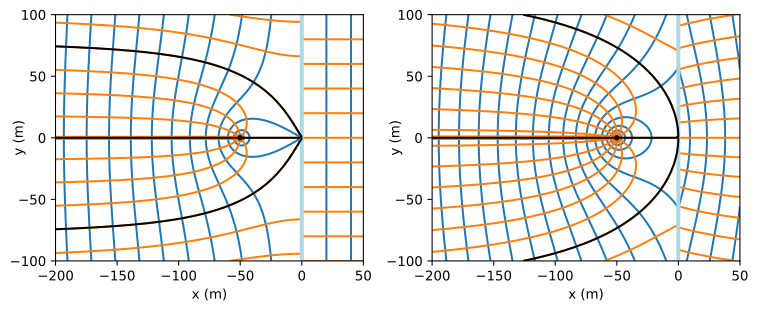
Figure 7.11 Flow net for a well pumping at critical pumping rate in uniform background flow near a river with zero bed resistance (\(C=\infty\), left) and non-zero bed resistance (\(C=0.5\) m\(^2\)/d, right); the capture zone envelopes are shown in black.

      When the discharge of the well is larger than \(Q_\text{cr}\), the well may draw water from the river, or it may draw water from the other side of the river, or both. This means that there is a section of river near the well, where water on the left side of the river flows towards the well. The points on the river where flow in the aquifer changes from towards the river to away from the river are obtained numerically. The function func2 returns the \(Q_x\) component of the discharge vector just on the left side of the river for given \(y\) and \(Q\) values. The brentq function is used again to find the change point where func2 equals zero. Note that for this case with river bed resistance, the change point is not a stagnation point, as \(Q_y\) does not equal zero. The change point is computed for the case that \(Q=2Q_{cr}\) as follows

# changed parameters
Q = 2 * Qcr2

# solution
def func2(ys, Q):
    return Qxriverleft(Q, ys)

ys = brentq(func2, 0, 2 * d, args=(Q))
print(f'point on the river where Qx equals zero: {ys:.2f} m')

point on the river where Qx equals zero: 57.44 m

      The flow net is shown in Figure 7.12. The code to produce the flow net is similar to the code for Figure 7.11. and is not repeated. The capture zone extends to the right side of the river. Whether the well captures water from the river or from the right side of the river is determined by the head in the aquifer at the river. If the head in the aquifer at the river is above the water level in the river \((h_R=10\) m), then water flows from the aquifer into the river. If the head in the aquifer at the river is below the water level in the river, then water flows from the river into the aquifer. For the values used in this example, the head in the aquifer at the origin is above the water level in the river, so that the well captures water from the other side of the river, but not from the river itself.

print(f'head at origin: {omegaresriv(0, 0, Q).real / T:.2f} m')
print(f'head at well: {omegaresriv(-d + rw, 0, Q).real / T:.2f} m')

head at origin: 10.25 m
head at well: 9.87 m

Figure 7.12 Flow net and capture zone envelope (black) for a well in uniform background flow near a river with a leaky bed; discharge between two streamlines is \(\Delta\Psi=2\) m\(^3\)/d. The riverbed conductance is \(C=0.5\) m\(^2\)/d and the critical discharge is \(Q_{cr}=25.54\) m\(^2\)/d. The well draws water from the right side of the river when \(Q>Q_{cr}\) for this case.

Exercise 7.11

Consider the example with streambed resistance presented above. Compute the head along the river for the case that the discharge of the well equals zero.

Solution

\(h=10.4\) m