1.4. Flow through two zones of different transmissivities

In the previous solutions, the hydraulic conductivity and saturated thickness were approximated as constant. Here, the aquifer consists of two zones of different, but constant transmissivities (Figure 1.15). The one-dimensional confined flow is between two parallel rivers with specified heads. The rivers are a distance \(L\) apart. The zone on the left has length \(L_0\), hydraulic conductivity \(k_0\), and thickness \(H_0\). The zone on the right has length \(L_1\), hydraulic conductivity \(k_1\), and thickness \(H_1\). Hence, the transmissivity in the left zone is \(T_0 = k_0 H_0\) and the transmissivity in the right zone is \(T_1 = k_1 H_1\). Recall that the general solution for the head in a confined aquifer (Eq. (1.9)) was derived for a constant transmissivity. The solution is valid in zone 0 and in zone 1, but with different integration constants. For \(N = 0\), the solution in zone 0 is

(1.46)\[ h=A_0x +B_0 {\hskip 2em} \text{zone 0} \]

and in zone 1

(1.47)\[ h=A_1x +B_1 {\hskip 2em} \text{zone 1} \]

where \(A_0\), \(A_1\), \(B_0\), and \(B_1\) are constants to be determined from boundary conditions.

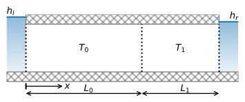
Figure 1.15 Confined flow through two zones of different transmissivities.

      There are two boundary conditions and two continuity conditions, because the head and flow are continuous across the boundary between zones 0 and 1

(1.48)\[ h\vert_{x=0}=h_l \]

(1.49)\[ h\vert_{x=L}=h_r \]

(1.50)\[ h|_{x=L_0^-}=h|_{x=L_0^+} \]

(1.51)\[ Q_x|_{x=L_0^-}=Q_x|_{x=L_0^+} \]

where the superscripts \(^+\) and \(^-\) stand for evaluation just to the left and just to the right of \(x = L_0\), respectively. Application of these four conditions and a bit of algebra gives the head solution

(1.52)\[ h=\frac{T_1L}{T_0L_1 + T_1L_0}\frac{(h_r-h_l)}{L}x + h_l \hskip 2em \text{zone 0} \]

(1.53)\[ h=\frac{T_0L}{T_0L_1 + T_1L_0}\frac{(h_r-h_l)}{L}(x-L) + h_r \hskip 2em \text{zone 1} \]

and the flow solution

(1.54)\[ Q_x=-\frac{T_0T_1L}{T_0L_1 + T_1L_0}\frac{(h_r-h_l)}{L} \hskip 2em \text{zones 0 and 1} \]

The discharge vector is once again constant for this solution (because \(N = 0\)), so the amount of water that flows into the aquifer on the left must discharge into the river on the right.
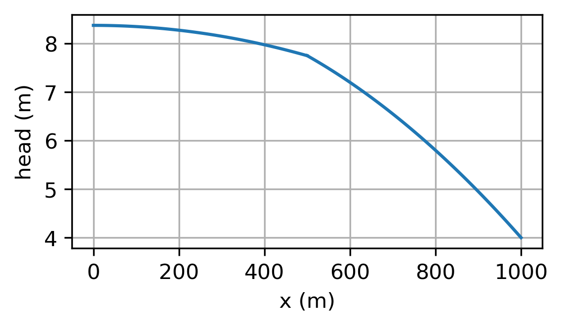
      The head function consists of two straight segments (Figure 1.16). The head gradient is smaller in the zone with the larger transmissivity and the head gradient is larger in the zone with the smaller transmissivity such that the product of the transmissivity and the head gradient is equal for both zones. In the example below, the aquifer is divided in two halves (\(L_0 = L_1\)) and the transmissivity of the left half of the aquifer is 10 times larger than the transmissivity of the right half of the aquifer. As a result, the head gradient is 10 times smaller in the left zone as compared to the right zone.

# parameters
hl = 6 # specified head at the left boundary, m
hr = 4 # specified head at the right boundary, m
L0 = 500 # length of zone 0, m
L1 = 500 # length of zone 1, m
T0 = 200 # transmissivity of zone 0, m^2/d
T1 = 20 # transmissivity of zone 1, m^2/d
L = L0 + L1 # total length, m

# solution
x = np.linspace(0, L, 101)
h = np.empty_like(x)
h[x < L0] = T1 * L / (T0 * L1 + T1 * L0) * (hr - hl) * x[x < L0] / L + hl
h[x >= L0] = T0 * L / (T0 * L1 + T1 * L0) * (hr - hl) * (x[x >= L0] - L) / L + hr
Qx = -T0 * T1 * L / (T0 * L1 + T1 * L0) * (hr - hl) / L 
hhalfway = h[50]
print(f'head halfway: {hhalfway:.2f} m')
print(f'head gradient zone 0: {(hhalfway - hl) / L0: .6f}')
print(f'head gradient zone 1: {(hr - hhalfway) / L1: .6f}')

head halfway: 5.82 m
head gradient zone 0: -0.000364
head gradient zone 1: -0.003636

# basic plot
plt.subplot(121)
plt.plot(x, h)
plt.subplot(122)
plt.plot([0, L], [Qx, Qx]);

Figure 1.16 Confined flow through two zones of different transmissivities; head (left) and \(Q_x\) (right).

      The solution for \(Q_x\) (Eq. (1.54)) is compared with the solution for a homogeneous aquifer with transmissivity \(T\) (Eq. (1.15)), which shows that the transmissivity of the two zones may be replaced by a single effective transmissivity \(T_\text{eff}\) for the whole aquifer that results in the correct flow rate

(1.55)\[ T_\text{eff} = \frac{T_0 T_1 L}{T_0 L_1 + T_1 L_0} = \frac{L}{L_1/T_1 + L_0/T_0} \]

The effective transmissivity is equal to the harmonic mean of the transmissivities of each zone, weighted by the zone lengths. The harmonic mean is commonly (much) smaller than the arithmetic mean.

print(f'arithmetic mean transmissivity: {(T0 + T1) / 2: .1f} m^2/d')
print(f'effective transmissivity: {L / (L1 / T1 + L0 / T0): .1f} m^2/d')

arithmetic mean transmissivity:  110.0 m^2/d
effective transmissivity:  36.4 m^2/d

Exercise 1.10

Compute the travel time from the left river to \(x = L_0\) and from \(x = L_0\) to \(x = L\) using that the thickness of both zones is 10 m and the porosity of both zones is 0.3. Repeat the computation for the case that \(H_0 = 10\) m and \(H_1 = 5\) m, while still using the same value of \(T_1\).

Solution

For \(H_0 = H_1 = 10\) m:
\(t = 20625\) d from \(x=0\) to \(x = L_0\)
\(t = 20625\) d from \(x=L_0\) to \(x = L\)

For \(H_0 = 10\) m and \(H_1 = 5\) m:
\(t = 20625\) d from \(x=0\) to \(x = L_0\)
\(t = 10312\) d from \(x=L_0\) to \(x = L\)

Exercise 1.11

Consider the same case as the example, but now the left boundary is impermeable, and there is a uniform areal recharge of \(N = 0.001\) m/d over the entire aquifer. \(T_1 = 100\) m\(^2\)/d, and all other values are as in the example. First, derive an equation for the head between \(x = L_0\) and \(x = L\) and compute the head at \(x = L_0\). Then derive an equation for the head between \(x = 0\) and \(x = L_0\). Plot the head vs. \(x\).

Solution

\(h|_{x=L_0} = 7.75\) m