1.1. Flow between two rivers

The first problem that is solved is for confined flow between two long and parallel rivers that fully penetrate the aquifer (Figure 1.2). The rivers are a distance \(L\) apart, and there is no areal recharge (\(N=0\)). The rivers are in direct contact with the aquifer so that the head in the aquifer at the river is equal to the head in the river. The head at \(x=0\) is \(h_l\), and the head at \(x=L\) is \(h_r\).

(1.10)\[ h\vert_{x=0} = h_l \]

(1.11)\[ h\vert_{x=L} = h_r \]

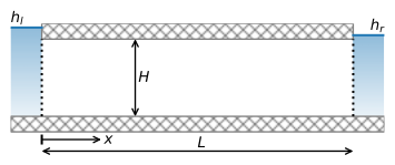
Figure 1.2 Flow between two rivers.

      Application of the boundary conditions to the general solution (1.9) gives

(1.12)\[ A=\frac{h_r-h_l}{L} \]

(1.13)\[ B=h_0 \]

so that the solution for the head becomes a straight line

(1.14)\[ h=\frac{(h_r-h_l)x}{L} + h_l \]

The discharge vector \(Q_x\) is obtained by differentiating Eq. ((1.14)) with respect to \(x\) and inserting the result into Eq. ((1.6))

(1.15)\[ Q_x = -T\frac{\text{d}h}{\text{d}x} = - T\frac{h_r-h_l}{L} \]

Note that \(Q_x\) is constant throughout the flow field.
      The solution is computed below and plotted in Figure 1.3. For the novice Python user, please be aware that the code blocks below only run when the numpy and matplotlib.pyplot packages are imported first as np and plt, respectively. This holds for virtually all code blocks in this book; see Appendix A for more details. Note that the porosity \(n\) and elevation \(z_b\) of the bottom of the aquifer are defined but not used here. They will be used when visualizing the flow field and computing the travel time in the following.

# parameters
L = 1000 # aquifer length, m
H = 10 # aquifer thickness, m
zb = -6 # aquifer bottom, m
k = 10 # hydraulic conductivity, m/d
n = 0.3 # porosity, -
T = k * H # transmissivity, m^2/d
hl = 6 # specified head at the left boundary, m
hr = 4 # specified head at the right boundary, m

# solution
x = np.linspace(0, L, 100)
h = (hr - hl) * x / L + hl
Qx = - T * (hr - hl) / L * np.ones_like(x)

# basic plot
plt.subplot(121)
plt.plot(x, h)
plt.subplot(122)
plt.plot(x, Qx);

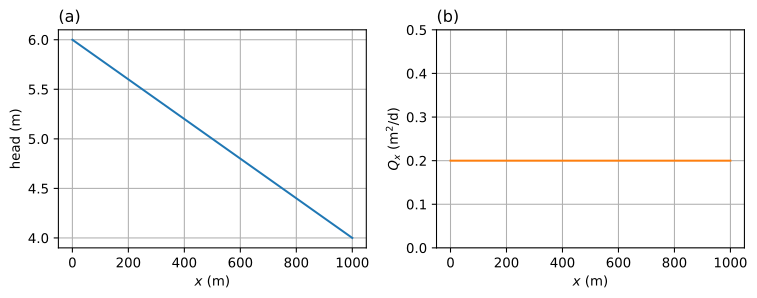
Figure 1.3 Flow between two rivers with \(N=0\); head (left) and \(Q_x\) (right).

      The flow field in a vertical cross-section may be visualized using the streamplot function of matplotlib, which takes as input a two-dimensional grid of points, and for each grid point, the horizontal and vertical components of the specific discharge vector. The horizontal component of the specific discharge vector \(q_x\) is computed from the discharge vector \(Q_x\) as

(1.16)\[ q_x = \frac{Q_x}{H} = -k\frac{h_r - h_l}{L} \]

and does not vary in the vertical direction. The vertical component of the specific discharge vector \(q_z\) equals zero. The streamplot function draws lines in the direction of the flow and adds arrows to indicate the direction of flow. For this case with constant flow, a small grid of 2 by 2 is sufficient. The vertical exaggeration is set with the aspect keyword of the subplot function. The vertical exaggeration is noted as “VE” in the label of the vertical axis (Figure 1.4).

# solution
xg, zg = np.meshgrid(np.linspace(0, L, 2), np.linspace(zb, zb + H, 2))
qx = -k * (hr - hl) / L * np.ones_like(xg)
qz = np.zeros_like(xg)

# basic stream plot
plt.subplot(111, aspect=25)
plt.streamplot(xg, zg, qx, qz, color='C1', density=0.2);

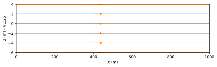
Figure 1.4 Streamplot in a vertical cross-section for flow between two rivers with \(N=0\).

      The (average) velocity in the horizontal direction \(v_x\) is obtained through division of \(q_x\) by the porosity \(n\) (obviously, the velocity in the vertical direction \(v_z\) is zero). For this simple problem,the (average) travel time from the left river to the right river can be computed as \(L/v_x\). More formally, the travel time can be obtained from the definition of the horizontal velocity vector

(1.17)\[ v_x = \frac{q_x}{n} = \frac{\text{d}x}{\text{d}t} \]

Integration gives the travel time \(t_\text{tr}\)

(1.18)\[ \int_0^{t_\text{tr}} \text{d}t = \int_{0}^L \frac{\text{dx}}{v_x} = \int_{0}^L -\frac{Ln}{k(h_r-h_l)}\text{d}x \]

which gives

(1.19)\[ t_\text{tr} = \frac{L^2n}{k(h_l-h_r)} = \frac{L}{v_x} \]

# travel time
vx = -k * (hr - hl) / (n * L)
print(f'mean velocity: {vx:.4f} m/d')
print(f'travel time from left river to right river: {L / vx:.0f} days')

mean velocity: 0.0667 m/d
travel time from left river to right river: 15000 days