4.2. Unconfined interface flow

Consider steady unconfined interface flow in a coastal aquifer as shown in Figure 4.4. The head and elevations are again measured with respect to sea level. The bottom of the aquifer is at \(z=z_b\). As for confined flow, unconfined flow in coastal aquifers may consist of a part near the shore where the interface is present and a part of the aquifer farther inland where there is no interface. The problem is again solved in terms of a discharge potential in both parts of the aquifer.

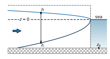
Figure 4.4 Steady interface flow in an unconfined aquifer.

      First, consider the freshwater zone above the interface. The water table is a distance \(h\) above sea level, and the elevation of the interface is obtained with the Ghyben–Herzberg equation ((4.4)) as \(z_i=-\alpha h\) so that the total thickness of the freshwater zone is equal to \(h-z_i=(1+\alpha)h\). The discharge vector may be written as

(4.22)\[ Q_x = -k(\alpha+1)h\frac{\text{d}h}{\text{d}x}= -\frac{\text{d}\Phi}{\text{d}x} \]

where the discharge potential for unconfined interface flow is

(4.23)\[ \Phi = \tfrac{1}{2}k(\alpha+1)h^2 {\hskip 2em} 0\le h \le -z_b/\alpha \]

Second, consider the part of the flow upstream of the toe, where the flow is unconfined without an interface. The saturated thickness is equal to \(h - z_b\) (recall that the head is measured with respect to the sea level) so that the discharge vector may be written as

(4.24)\[ Q_x = -k(h-z_b)\frac{\text{d}h}{\text{d}x}= -\frac{\text{d}\Phi}{\text{d}x} \]

where the discharge potential is

(4.25)\[ \Phi = \tfrac{1}{2}k(h-z_b)^2 + C_u {\hskip 2em} h\ge -z_b/\alpha \]

The constant \(C_u\) is chosen such that the potential is continuous at the point where the flow changes from unconfined interface flow to regular unconfined flow, which is at the toe of the interface. The head at the toe is equal to \(h_\text{toe}=-z_b/\alpha\), and the potential at the toe of the interface may be computed with Eq. ((4.23)) as

(4.26)\[ \Phi_\text{toe} = \tfrac{1}{2}k\frac{\alpha+1}{\alpha^2}z_b^2 \]

Constant \(C_u\) is obtained by setting the discharge potential (Eq. (4.25)) equal to \(\Phi_\text{toe}\), with \(h=-z_b/\alpha\) at the toe

(4.27)\[ \Phi_\text{toe} = \frac{1}{2}k\left(-\frac{z_b}{\alpha}-z_b\right)^2 + C_u=\tfrac{1}{2}k\frac{\alpha+1}{\alpha^2}z_b^2 \]

so that

(4.28)\[ C_u = -\tfrac{1}{2}k\frac{\alpha+1}{\alpha}z_b^2 \]

As for confined interface flow, head-specified boundary conditions need to be transformed into discharge potentials using either Eq. ((4.23)) or ((4.25)), depending on the value of the head. Once a solution is obtained in terms of the discharge potential, the head may be computed with the inverse of Eq. ((4.23)) or ((4.25))

(4.29)\[ h=\sqrt{\frac{2\Phi}{k(\alpha + 1)}} {\hskip 2em} \Phi \le \Phi_\text{toe} \]

(4.30)\[ h = \sqrt{\frac{2(\Phi-C_u)}{k}} + z_b {\hskip 2em} \Phi \ge \Phi_\text{toe} \]

As an example, consider unconfined interface flow in a cross section of a long strip island. The distance between the two shores (i.e., the width of the island) is \(L\), and the infiltration rate is equal to \(N\). The origin of the coordinate system is chosen at the left coast (Figure 4.5). At both coasts, the head is equal to sea level

(4.31)\[ h\vert_{x=0} = h\vert_{x=L} = 0 \]

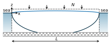
Figure 4.5 Unconfined interface flow below an infinite strip island with areal recharge.

The corresponding boundary conditions in terms of potentials are

(4.32)\[ \Phi\vert_{x=0} = \Phi\vert_{x=L} = 0 \]

The potential as a function of \(x\) for this case was derived in Section 3.3. Substitution of boundary conditions ((4.32)) in Eq. ((3.39)) gives

(4.33)\[ \Phi=-\frac{N}{2}(x^2 - Lx) \]

The interface reaches the bottom of the aquifer when the potential at the center of the island is larger than the potential at the toe \(\Phi_\text{toe}\) (Eq. (4.26)). In the example below, the solution is plotted for two values of the recharge \(N\): one value for which the interface doesn’t reach the bottom of the aquifer and one value for which the interface reaches the bottom of the aquifer (Figure 4.6).

# parameters
k = 40 # hydraulic conductivity, m/d
zb = -20 # bottom of aquifer, m
rhof = 1000 # density of fresh water, kg/m^3
rhos = 1025 # density of salt water, kg/m^3
L = 1000 # width of island, m
N1 = 0.001 # recharge rate 1, m/d
N2 = 0.002 # recharge rate 2, m/d
alpha = rhof / (rhos - rhof) # alpha factor

# solution
def pot(x, N, L):
    phi = -0.5 * N * (x**2 - L * x)
    return phi

def pot2h(pot, k, alpha, zb):
    phitoe = 0.5 * k * (alpha + 1) / alpha**2 * zb**2
    Cu = -0.5 * k * (alpha + 1) * zb**2 / alpha
    h = np.zeros(len(pot))
    h[pot < phitoe] = np.sqrt(2 * pot[pot < phitoe] / (k * (alpha + 1)))
    h[pot >= phitoe] = np.sqrt(2 * (pot[pot >= phitoe] - Cu) / k) + zb
    return h

def zinterface(h, alpha, zb):
    return np.maximum(-alpha * h, zb)

x = np.linspace(0, L, 201)
phi1 = pot(x, N1, L)
phi2 = pot(x, N2, L)
h1 = pot2h(phi1, k, alpha, zb)
h2 = pot2h(phi2, k, alpha, zb)
zi1 = zinterface(h1, alpha, zb)
zi2 = zinterface(h2, alpha, zb)

phitoe = 0.5 * k * (alpha + 1) / alpha**2 * zb**2
print(f'Phi_toe: {phitoe:.2f}')
print(f'N={N1} results in maximum phi {np.max(phi1)}')
print(f'N={N2} results in maximum phi {np.max(phi2)}')

Phi_toe: 205.00
N=0.001 results in maximum phi 125.0
N=0.002 results in maximum phi 250.0

# basic plot
plt.subplot(111, aspect=10)
plt.plot(x, zi1, label=f'N={N1} m/d')
plt.plot(x, zi2, label=f'N={N2} m/d')
plt.legend();

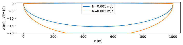
Figure 4.6 Unconfined interface flow in a cross section of an infinite strip island.

      When the recharge rate is large enough, the location of the toe of the interface may be obtained by setting \(\Phi=\Phi_\text{toe}\) and solving for \(x\), which gives

(4.34)\[ x_\text{toe} = \frac{L}{2} \pm \frac{1}{2}\sqrt{L^2 - \frac{8\Phi_\text{toe}}{N}} \]

If the recharge is too small, the argument of the square root is negative and the interface does not reach the bottom of the aquifer. The location of the toe of the interface is a function of the sea level, because the equation for \(\Phi_\text{toe}\) contains the elevation \(z_b\) of the base of the aquifer. Recall that \(z_b\) is measured with respect to the sea level. So when the sea level rises by 1 m, that means that \(z_b\) is 1 m lower than without the sea level rise.
      Streamlines for the case with the larger recharge rate (\(N = 2\) mm/d) are shown below (Figure 4.7). As for confined flow, the simulated length of the outflow zone is zero, as a result of the Dupuit approximation. This same problem is solved for a horizontal sea floor without the Dupuit approximation in Section 10.6, which results in an outflow zone along the bottom of the sea.

# solution
xg = [x, x]
zg = [zi2, h2]
psi = [np.zeros_like(x), N2 * (x - L / 2)]

# basic streamline plot
plt.subplot(111, aspect=10)
plt.contour(xg, zg, psi, 20);

Figure 4.7 Streamlines for unconfined interface flow in a vertical cross section of an infinite strip island with areal recharge \(N\)Discharge between two streamlines is \(\Delta\psi=0.1\) m\(^2\)/d.

Exercise 4.5

Compute the locations of the toes of the interface for the case that \(N = 0.002\) m/d and all other parameters are as in the example. Next, compute the locations of the toes of the interface for the case that the sea level rises by 1 m.

Solution

\(x_\text{toe} = 500 \pm 212.13\) m before sea level rise.
\(x_\text{toe} = 500 \pm 154.88\) m after sea level rise.

Exercise 4.6

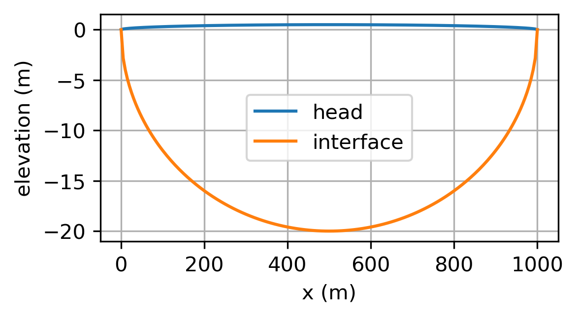
For the example above, compute the recharge \(N\) such that the interface exactly touches the bottom of the aquifer at \(x = 500\) m. Plot the head and interface vs \(x\).

Solution

\(N = 0.00164\) m/d

Exercise 4.7

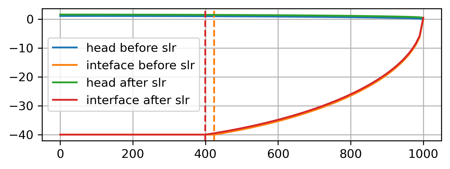
Compute and plot the elevation of the interface for the case of unconfined interface shown in Figure 4.8. Use \(k = 20\) m/d, \(N = 0.001\) m/d, \(\rho_s=1025\) kg/m\(^3\), \(z_b=-40\) m, \(L=1000\) m. Compute the head at \(x = 0\) and the location of the toe of the interface. Compare your answer for the head at \(x = 0\) to the same problem of regular unconfined flow (all freshwater).

Solution

\(h_0 = 1.11\) m with interface
\(h_0 = 0.62\) m without interface

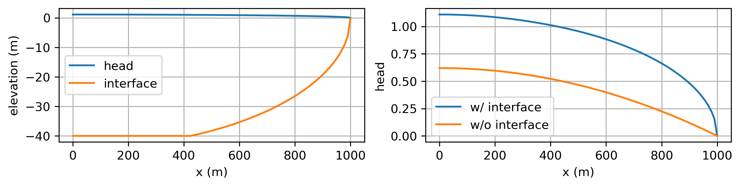
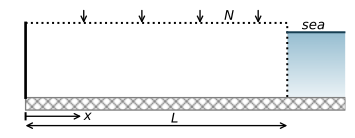
Figure 4.8 Situation for Exercise 4.7.

Exercise 4.8

Reconsider the case of Exercise 4.7. Compute the location of the toe when the sea level rises by 0.5 m and all the other parameters remain the same. Plot the head vs. \(x\), using the original sea level as a datum. Compute the change in the position of the toe after the sea level rise.

Solution

Toe moves inland 25.05 m after sea level sea