3.3. Combined confined/unconfined flow with areal recharge

So far in this chapter, separate solutions have been derived for confined flow (or flow with constant transmissivity) and unconfined flow. In this section, a case is considered where the flow changes from confined flow to unconfined flow somewhere in the aquifer. Consider flow between two parallel rivers in a confined aquifer with thickness \(H\) (Figure 3.9); the rivers are in direct contact with the aquifer. The rivers are a distance \(L\) apart, and the areal recharge is uniform and equal to \(N\). The stage \(h_l\) in the left river is above the top of the aquifer, and the stage \(h_r\) in the right river is below the top of the aquifer. Hence, groundwater flow is confined near the left river, is unconfined near the right river, and changes somewhere in the aquifer from confined to unconfined.

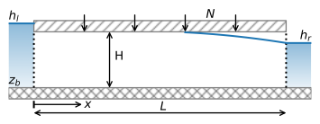
Figure 3.9 Combined confined/unconfined flow between two rivers.

     One approach to solving this problem is to write one solution for the head in the confined part of the aquifer and a separate solution for the head in the unconfined part and then try to find the point where flow changes from confined to unconfined. This is possible, but the use of the discharge potential provides an easier way. The discharge potential was already defined for unconfined flow, but not yet for confined flow. For confined flow, the discharge vector may be written as

(3.30)\[ Q_x=-kH\frac{\text{d}h}{\text{d}x}=-\frac{\text{d}}{\text{d}x}(kHh)=-\frac{\text{d}\Phi}{\text{d}x} \]

where both \(k\) and \(H\) are constant. The discharge potential for confined flow is defined as

(3.31)\[ \Phi = kHh + C \]

where \(C\) is an arbitrary constant. When the flow is purely confined, the constant \(C\) can be set to zero, but when the flow is confined in parts of the aquifer and unconfined in other parts of the aquifer, the constant \(C\) must be picked differently, as explained in the following.
     Now that both confined flow and unconfined flow are formulated as potential flow, the discharge vector may be written as Eq. ((3.3)) , the governing differential equation is the Poisson equation ((3.5)), and the general solution for one-dimensional steady potential flow is Eq. ((3.6)). This means that the discharge potential is a continuous function of \(x\), irrespective of whether the flow is confined or unconfined. The discharge potential must be converted to a head that is also a continuous function of \(x\) (as the head cannot suddenly jump up or down without a physical barrier to flow). This is achieved by proper selection of the constant \(C\) in Eq. ((3.31)). At the point where the flow transitions from confined to unconfined, the head in the aquifer is equal to \(z_b+H\). The potential at this point is referred to as the transition potential \(\Phi_t\) and may be computed from the potential for unconfined flow (Eq. (3.2)) as

(3.32)\[ \Phi_t = \tfrac{1}{2}kH^2 \]

The constant \(C\) is chosen such that the discharge potential for confined flow yields the same transition potential

(3.33)\[ \Phi_t = kH(z_b + H) + C = \tfrac{1}{2}kH^2 \]

so that

(3.34)\[ C=-\tfrac{1}{2}kH^2 - kHz_b \]

     Once the discharge potential is computed as a function of \(x\), it is converted to a head using the appropriate equation. If the flow is confined,

(3.35)\[ h=\frac{\Phi-C}{kH} \hskip 2em \Phi\ge\Phi_t \]

and if the flow is unconfined

(3.36)\[ h = z_b + \sqrt{2\Phi/k} \hskip 2em \Phi\le\Phi_t \]

     As an example, the problem of Section 1.2 is solved, but now the thickness of the aquifer is fixed to \(H\) while the saturated thickness of the aquifer may vary with the head. The boundary conditions are

(3.37)\[ \Phi\vert_{x=0}=\Phi_l=kHh_l + C \]

(3.38)\[ \Phi\vert_{x=L}=\Phi_r=\tfrac{1}{2}k(h_r-z_b)^2 \]

Application of the boundary conditions to the general solution (3.6) gives

(3.39)\[ \Phi = -\frac{N}{2}(x^2 - Lx) + \frac{(\Phi_r - \Phi_l)x}{L} + \Phi_0 \]

The head solution is obtained from the potential with Eq. ((3.35)) or ((3.36)). Results for the same parameters as Section 1.2 are shown in Figure 3.10. Note that the flow is unconfined for only a small section of the aquifer near the right river.

# parameters
L = 1000 # aquifer length, m
H = 10 # aquifer thickness, m
zb = -5 # aquifer base, m
k = 10 # hydraulic conductivity, m/d
hl = 6 # specified head at the left boundary, m
hr = 4 # specified head at the right boundary, m
N = 0.001  # areal recharge, m/d

# solution
C = -0.5 * k * H**2 - k * H * zb
phil = k * H * hl + C
phir = 0.5 * k * (hr - zb)**2
phit = 0.5 * k * H**2  # transition potential
x = np.linspace(0, L, 400)
phi = -N / 2 * (x ** 2 - L * x) + (phir - phil) * x / L + phil
h = np.zeros_like(phi)
h[phi >= phit] = (phi[phi > phit] - C) / (k * H)
h[phi <= phit] = zb + np.sqrt(2 * phi[phi <= phit] / k)
Qx = N * (x - L / 2) - (phir - phil) / L 
happrox = -N / (2 * k * H) * (x ** 2 - L * x) + (hr - hl) * x / L + hl
Qxapprox = N * (x - L / 2) - k * H * (hr - hl) / L 

# basic plot
plt.subplot(121)
plt.plot(x, h, 'C0')
plt.plot(x, happrox, 'C0--')
plt.subplot(122)
plt.plot(x, Qx, 'C1')
plt.plot(x, Qxapprox, 'C1--')

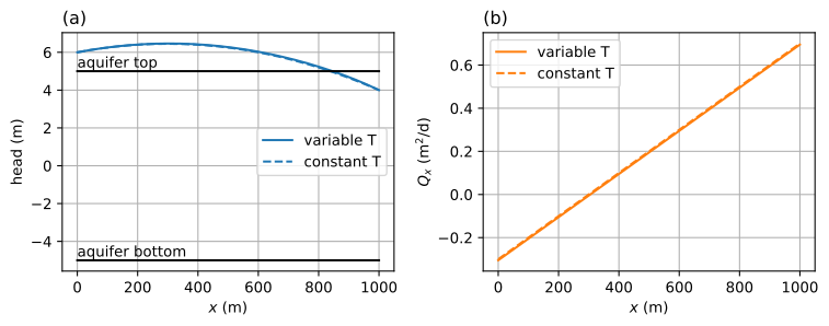
Figure 3.10 Combined confined/unconfined flow; head (left) and \(Q_x\) (right).

     The flux into the left river is now slightly higher than in Section 1.2, while the flux into the right river is slightly lower, so that the sum of the outflow in the two rivers is still equal to \(NL\).

print(f'flux to left river: {-Qx[0]:.3f} m^2/d')
print(f'flux to right river: {Qx[-1]:.3f} m^2/d')

flux to left river: 0.305 m^2/d
flux to right river: 0.695 m^2/d

     A contour plot of the steam function is created below (Figure 3.11). The top of the saturated zone is formed by the top of the aquifer in the zone where the flow is confined, and by the water table in the zone where the flow is unconfined.

# solution
psi = np.zeros((2, len(x)))
psi[1] = -Qx
xg = np.zeros_like(psi)
xg[:] = x
zg = np.zeros_like(psi)
zg[0] = zb
zg[1] = H + zb
zg[1, h < H + zb] = h[h < H + zb]

# basic streamline plot
plt.subplot(111, aspect=25)
plt.contour(xg, zg, psi, 20, colors='C1', linestyles='-')
plt.plot(xg[0], zg[1], 'C0');

Figure 3.11 Streamlines in a vertical cross section for combined confined/unconfined flow. Discharge between two streamlines is \(\Delta\psi=0.05\) m\(^2\)/d.

Exercise 3.5

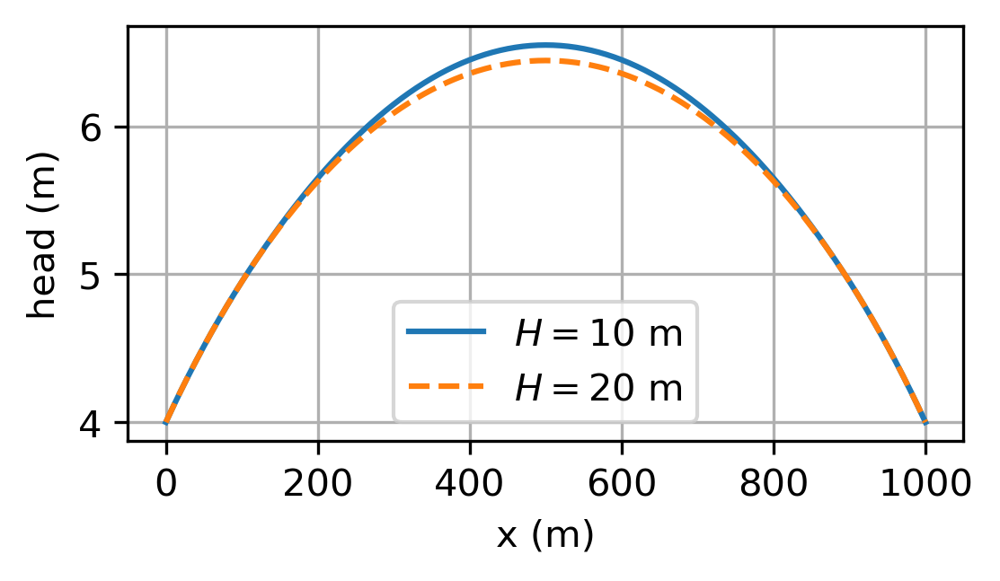
Consider the case that \(h_l=h_r=4\) m and \(N=0.002\) m/d. All other parameters are as for the example above, except for the aquifer thickness. Compute the head halfway between the two rivers for \(H=10\) m and for \(H=20\) m. Plot the head as a function of \(x\) for both cases in the same graph.

Solution

\(h=6.550\) m for \(H=10\) m
\(h=6.446\) m for \(H=20\) m