4.1. Confined interface flow

Consider steady interface flow in a confined coastal aquifer as shown in Figure 4.2. The elevations of the top and bottom of the aquifer are \(z_t\) and \(z_b\), respectively. The thickness of the aquifer is \(H=z_t-z_b\). Flow problems in coastal aquifers are commonly broken up into a part near the coast where the interface is present and a part upstream of the interface toe where there is no interface. The flow in both parts may be solved simultaneously by defining an appropriate discharge potential such that the flow may be computed in both parts of the aquifer as

(4.6)\[ Q_x = -\frac{\text{d}\Phi}{\text{d}x} \]

This was first done by Strack (1976), and these discharge potentials are also referred to as Strack potentials. Separate discharge potentials must be defined for the two parts of the flow system. Note that this approach is similar to the approach for combined confined/unconfined flow (Section 3.3), where separate discharge potentials were defined for the confined and the unconfined parts of the flow system.

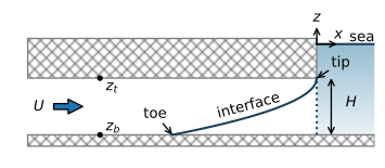
Figure 4.2 Interface flow toward the coast in a confined aquifer.

      First, consider the interface flow part. The elevation of the tip of the interface is at the top of the aquifer \(z_\text{tip} =z_t\), which corresponds to a head \(h_\text{tip}=-z_t/\alpha\). The elevation of the toe of the interface is \(z_\text{toe}=z_b\), which corresponds to a head \(h_\text{toe}=-z_b/\alpha\). Between the tip and the toe, the thickness of the freshwater zone is equal to \(z_t-z_i=z_t + \alpha h\). The discharge vector may be written as

(4.7)\[ Q_x = -k(z_t + \alpha h)\frac{\text{d}h}{\text{d}x} = -k\alpha(h+z_t/\alpha)\frac{\text{d}h}{\text{d}x} = -\frac{\text{d}\Phi}{\text{d}x} \]

so that the discharge potential is

(4.8)\[ \Phi = \tfrac{1}{2}k\alpha(h+z_t/\alpha)^2 {\hskip 2em} -z_t/\alpha\le h\le -z_b/\alpha \]

The potential \(\Phi_\text{toe}\) at the toe is obtained by substituting the head \(h_\text{toe}\) for \(h\) in Eq. ((4.8))

(4.9)\[ \Phi_\text{toe} = \frac{kH^2}{2\alpha} \]

Upstream of the toe, the flow is regular confined flow so that the saturated thickness is equal to \(H\) and the discharge vector may be written as

(4.10)\[ Q_x = -kH\frac{\text{d}h}{\text{d}x} = -\frac{\text{d}\Phi}{\text{d}x} \]

where the discharge potential is

(4.11)\[ \Phi = kHh + C_c {\hskip 2em} h\ge -z_b/\alpha \]

The constant \(C_c\) is chosen such that the discharge potential at the toe (where \(h_\text{toe}=-z_b/\alpha\)) is equal to \(\Phi_\text{toe}\) (Eq. (4.9))

(4.12)\[ \Phi_\text{toe} = -kHz_b/\alpha + C_c = \frac{kH^2}{2\alpha} \]

which gives

(4.13)\[ C_c = \frac{\tfrac{1}{2} kH^2 + kHz_b}{\alpha} \]

With this choice for \(C_c\), the potential is continuous when it transitions from regular confined flow to confined interface flow at the toe.
      Now that steady confined interface flow is written as potential flow, any potential flow solution may be used that fulfills the differential equation for steady one-dimensional potential flow (Eq. (3.5))

(4.14)\[ \frac{\text{d}^2\Phi}{\text{d}x^2}=-N \]

Head-specified boundary conditions need to be transformed into discharge potentials using either Eq. ((4.8)) or ((4.11)), depending on the value of the head. Once a solution is obtained in terms of the discharge potential, the head may be computed by the inverse of Eq. ((4.8)) or ((4.11))

(4.15)\[ h=\sqrt{\frac{2\Phi}{k\alpha}}-\frac{z_t}{\alpha} {\hskip 2em} \Phi \le \Phi_\text{toe} \]

(4.16)\[ h = \frac{\Phi-C_c}{kH} {\hskip 2em} \Phi \ge \Phi_\text{toe} \]

Finally, the elevation \(z_i\) of the interface may be computed from the head as

(4.17)\[ z_i = -\alpha h {\hskip 2em} h_\text{tip} \le h \le h_\text{toe} \]

As an example, consider uniform flow toward the coast at a rate \(Q_x = U\) as shown in Figure 4.2 (\(Q_x\) is constant because the recharge \(N = 0\)). The origin of the coordinate system is chosen at the coastline, and the aquifer extends toward negative infinity. The elevation of the top of the confined aquifer is \(z_t\) with respect to sea level. The head at the coastline is \(-z_t/\alpha\), which is equivalent to an interface elevation of \(z_i=z_t\). The corresponding discharge potential at the coastline is obtained by substituting \(h=-z_t/\alpha\) in the equation for the discharge potential (Eq. (4.8)), which gives \(\Phi=0\). Hence, the boundary conditions are

(4.18)\[ \Phi\vert_{x=0}=0 \]

(4.19)\[ Q_x=-\frac{\text{d}\Phi}{\text{d}x}=U \]

The solution for the potential that fulfills the differential equation ((4.14)) with \(N=0\) and the boundary conditions is

(4.20)\[ \Phi = -Ux \]

The location of the toe is found at the position where \(\Phi=\Phi_\text{toe}\), which gives

(4.21)\[ x_\text{toe}=-\frac{\Phi_\text{toe}}{U}=-\frac{kH^2}{2\alpha U} \]

Note that for a given value of \(U\), the location of the toe is a function only of the aquifer parameters \(k\) and \(H\), and the factor \(\alpha\), which is a function of the densities of freshwater and saltwater. The toe location is not a function of the sea level. And hence, the location of the toe remains where it is when the sea level rises, provided that the discharge toward the coast remains \(U\). The heads in the aquifer increase with the sea level rise, of course.
      In the example that follows, the location of the interface and the stream function are computed and plotted (Figure 4.3).

# parameters
k = 10 # hydraulic conductivity, m/d
zt = -10 # top of aquifer, m
zb = -30 # bottom of aquifer, m
rhof = 1000 # density of fresh water, kg/m^3
rhos = 1025 # density of salt water, kg/m^3
U = 0.4 # flow towards the coast, m^2/d
H = zt - zb # aquifer thickness, m

# solution
alpha = rhof / (rhos - rhof)
phitoe = 0.5 * k * H ** 2 / alpha
Cc = (0.5 * k * H ** 2 + k * H * zb) / alpha
x = np.linspace(-200, 0, 150)
phi = -U * x
h = np.zeros_like(phi)
h[phi <= phitoe] = np.sqrt(2 * phi[phi <= phitoe] / (k * alpha)) - zt / alpha
h[phi > phitoe] = (phi[phi > phitoe] - Cc) / (k * H)
zi = np.maximum(-alpha * h, zb)
#
xtoe = -k * H**2 / (2 * alpha * U)
print(f'x-location of the toe: {xtoe:.0f} m')
# stream function
xg = [x, x]
zg = [zi, zt * np.ones(len(x))]
psi = [np.zeros(len(x)), -U * np.ones(len(x))]

x-location of the toe: -125 m

# basic streamline plot
plt.subplot(111, aspect=2)
plt.contour(xg, zg, psi)
plt.plot(x, zi, 'C1');

Figure 4.3 Streamlines in a vertical cross section for uniform flow toward the coast (\(x = 0\)) in a confined coastal aquifer. Discharge between two streamlines is \(\Delta\psi=0.05\) m\(^2\)/d.

      The slopes of the streamlines change at the toe of the interface in Figure 4.3. This is a consequence of the Dupuit approximation. The tip of the interface is at the top of the aquifer at the coastline. This means that there is no gap for the freshwater to discharge into the sea. That is rather unrealistic and a consequence of adoption of the Dupuit approximation. For a coastline with a vertical beach face, as shown here with a dotted line, there is always a vertical outflow zone. The freshwater head varies along a vertical outflow zone, because the pressure distribution in the saltwater is hydrostatic, so that the freshwater head in the saltwater increases with depth. An example of two-dimensional interface flow in the vertical plane with an outflow zone along a horizontal sea bottom is presented in Section 10.5. Comparisons with interface solutions for two-dimensional flow in the vertical plane show that the location of the toe of the interface is often approximated reasonably well with a Dupuit solution, even though the depth of the interface near the coastline is underestimated (Sections 10.5 and 10.6).

Exercise 4.1

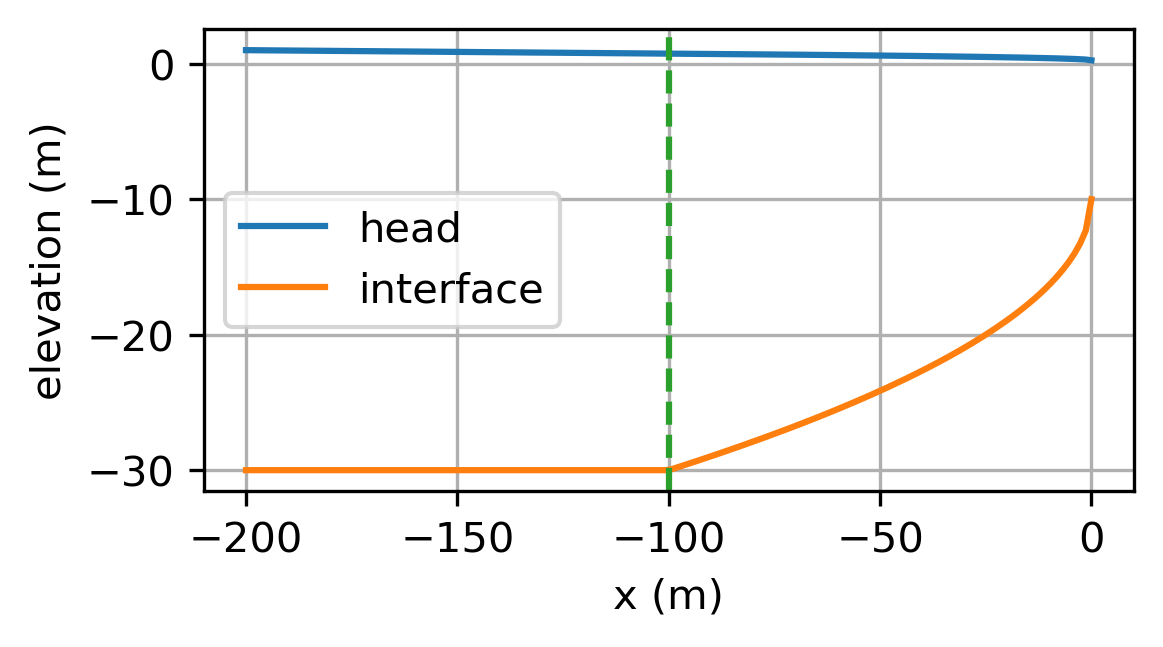
Redo the example for the case that the flow \(U\) is unknown, but the head is measured 200 m from the coastline and is equal to 1 m. Compute \(U\) and the location of the toe. Plot the head and interface vs. \(x\).

Solution

\(U = 0.5\) m\(^2\)/d, \(x_\text{toe} = -100\) m

Exercise 4.2

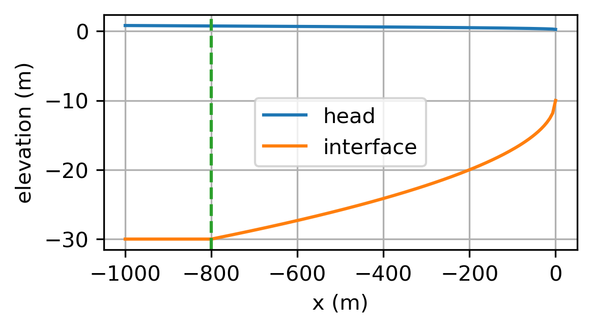
Redo the example for the case that the flow \(U\) is unknown, but the head is measured 200 m from the coastline and is equal to 0.5 m. Compute \(U\) and the location of the toe. Plot the head and interface vs. \(x\).

Solution

\(U = 0.06\) m\(^2\)/d, \(x_\text{toe} = -800\) m

Exercise 4.3

Reconsider the case of the example. Compute the location of the toe when the sea level rises by 0.5 m and all the other parameters remain the same. Compute the change in head in the aquifer.

Solution

Head increases by 0.5 m compared to original elevation. Interface remains at same elevation.

Exercise 4.4

Reconsider the case of Exercise 4.1. Compute the location of the toe when the sea level rises by 0.5 m while the head 200 m from the coastline remains the same. Note that the head 200 m from the coastline is measured with respect to the original sea level. What is the effect of sea level rise in a confined aquifer when the inland boundary is a specified head?

Solution

\(x_\text{toe} = -886\) m so the seawater intrusion increases.