10.3. Flow over a step in the base

The effect of a jump in the base on the flow and head distribution in an unconfined aquifer was investigated in Section 3.2 using a Dupuit solution. Here, the effect of a jump in the base on the flow and head distribution is investigated for confined flow using a solution for two-dimensional flow in the vertical plane. The two-dimensional flow solution is compared to a Dupuit solution and the effect of vertical anisotropy in the hydraulic conductivity is investigated. The solution is obtained with conformal mapping. This time, the function \(\zeta(\tau)\) can not be inverted analytically to get an expression for \(\tau(\zeta)\), which complicates evaluation of the function.
      Consider two-dimensional flow in the vertical plane in a confined aquifer with an impermeable top and an impermeable bottom. The base is piece-wise horizontal and jumps at \(x=0\) (see Figure 10.9). The aquifer thickness is equal to \(H_l\) for \(x\le 0\) and equal to \(H_r\) for \(x\ge 0\). The hydraulic conductivity is homogeneous and isotropic and equal to \(k\). Flow is equal to \(Q_x=U\) from the left to the right

(10.31)\[ \lim_{x\to -\infty}q_x H_l = \lim_{x\to \infty}q_x H_r = U \]

The stream function is chosen to equal \(\psi=0\) along the base of the aquifer, which means \(\psi=-U\) along the top of the aquifer. As a reference, the head is equal to zero at the origin

(10.32)\[ h_{x=0,z=0}=0 \]

      A solution to the stated problem is again sought in parametric form as \(\omega(\tau)\) and \(\zeta(\tau)\), where the reference plane \(\tau\) is chosen as the quarter plane shown in Figure 10.9. Point 1 is chosen to correspond to \(\tau=\infty\), point 2 corresponds to \(\tau=0\), and point 4 corresponds to \(\tau=1\); point 3 corresponds to \(\tau=\lambda\), where the value of \(\lambda\) is determined by the mapping. The top of the aquifer and the horizontal portions of the bottom of the aquifer correspond to the positive real axis of \(\tau\) (note the corresponding red, purple, and brown sections in the \(\zeta\) and \(\tau\) planes), while the vertical part of the bottom of the aquifer corresponds to the positive imaginary axis in the \(\tau\) plane (green).

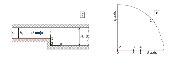
Figure 10.9 Flow over a step in the base; physical \(\zeta\) plane (left) and reference \(\tau\) plane (right).

      The solution to the stated problem is

(10.33)\[ \zeta = \frac{-H_r}{\pi}\ln\frac{\tau-\lambda}{\tau + \lambda} + \frac{H_l}{\pi}\ln\frac{\tau-1}{\tau + 1} + (H_r-H_l)i \]

(10.34)\[ \omega = \frac{-U}{\pi}\ln[(\tau-1)(\tau + 1)] + \frac{U}{\pi}\ln[(\tau-\lambda)(\tau + \lambda)/\lambda^2] \]

where \(\lambda=H_l/H_r\). Note the similarity between Eqs. ((10.33)) and ((10.20)), but for this case, as is common in conformal mapping, the solution \(\zeta(\tau)\) can not be inverted to obtain a solution \(\tau(\zeta)\). The solutions ((10.33)) and ((10.34)) are evaluated by selecting a value of \(\tau\) and evaluating both the complex potential \(\omega\) and the corresponding complex coordinate \(\zeta\).
      A flow net is created as follows. A grid is defined in the \(\tau\)-plane and both the complex coordinate \(\zeta=x+iz\) and the complex potential \(\omega\) are computed for each grid point. A contour plot is created using the regular contour function of matplotlib by passing it the computed irregular grid of \(x\) and \(z\) together with either the computed head or stream function.
      All points along the top of the aquifer (between points 3 and 4) correspond to the real axis of \(\tau\) between \(\xi=\lambda\) (point 3) and \(\xi=1\) (point 4). Some points that are far apart along the top of the aquifer in the \(\zeta\) plane are very close together in the \(\tau\)-plane. This phenomenon is called the crowding effect in conformal mapping. As a result, a regularly spaced grid in the \(\tau\) plane results in an irregular grid in the \(\zeta\) plane where some points may be very far apart. An accurate contour plot is obtained by defining an irregularly spaced grid in the \(\tau\) plane consisting of three segments in the \(\xi\) direction, from point 2 to 3, point 3 to 4, and point 4 to a large value; two segments are used in the \(\eta\) plane. Note that neither \(\zeta\) nor \(\omega\) can be computed easily at points 3 and 4, as the logarithms in the solution can not be evaluated at those points. The solution exists in the limit, of course. As a practical solution, the solution is evaluated up to a small distance from points 3 and 4, rather than mathematically taking the limit and programming the result.
      An example flow net is shown in Figure 10.10. The streamlines for the Dupuit solution are horizontal lines that jump at the base (compare Figure 3.8) and are shown with dashed lines in Figure 10.10. Note that the Dupuit streamlines are a good approximation of the two-dimensional streamlines beyond one aquifer thickness from the jump in the base. Similarly, the vertical head variation becomes negligible at approximately one aquifer thickness from the jump in the base.

# parameters
k = 10 # hydraulic conductivity, m/d
Hl = 10 # aquifer thickness on left side, m
Hr = 20 # aquifer thickness on right side, m
U = 0.1 # flow from left to right, m^2/d

# solution
def zetafunc(tau, Hr=Hr, Hl=Hl):
    lab = Hl / Hr
    zeta = -Hr / np.pi * np.log((tau - lab) / (tau + lab)) + \
            Hl / np.pi * np.log((tau - 1) / (tau + 1)) + \
           (Hr - Hl) * 1j
    return zeta

def omegafunc(tau, U=U, Hr=Hr, Hl=Hl):
    lab = Hl / Hr
    omega = -U / np.pi * np.log((tau - 1) * (tau + 1)) + \
             U / np.pi * np.log((tau - lab) * (tau + lab) / lab ** 2)
    return omega

# grid
d = 1e-14 # small offset
lab = Hl / Hr
xi1 = np.linspace(0, lab - d, 400)
xi2 = np.linspace(lab + d, 1 - d, 400)
xi3 = np.linspace(1 + d, 40, 400)
eta1 = np.linspace(0, 1, 400)
eta2 = np.linspace(1, 40, 400)
xi, eta = np.meshgrid(np.hstack((xi1, xi2, xi3)), np.hstack((eta1, eta2)))
zeta = zetafunc(xi + eta * 1j)
omega = omegafunc(xi + eta * 1j)

# basic plot
plt.subplot(111, aspect=1, xlim=(-20, 20))
plt.contour(zeta.real, zeta.imag, omega.real / k, np.arange(-0.1, 0.1, 0.002))
plt.contour(zeta.real, zeta.imag, omega.imag, np.arange(-0.1, 0, 0.02))
plt.plot([-40, 0, 0, 40], [10, 10, 0, 0], 'k');

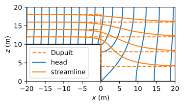
Figure 10.10 Flow net for confined flow with a jump in the base; head contour interval \(\Delta h= 2\) mm.

Exercise 10.2

Verify that the conformal mapping solution for \(\zeta\) (Eq. (10.33)) is correct by evaluating the solution at (or very close to) all corner points.

Solution

The solution is correct (-;

      Computation of the complex potential at a specific complex coordinate \(\zeta^*=x^* + iz^*\) in the aquifer requires a numerical approach the find the corresponding value of the parameter \(\tau\). For example, \(\tau\) can be found by minimizing the function

(10.35)\[ f(\tau) = (x^* - x(\tau))^2 + (z^* - z(\tau))^2 \]

Minimization can be carried out with a standard non-linear minimization routine such as the fmin function of scipy.optimize. fmin searches for an array of real variables that minimizes a function, so \(\xi\) and \(\eta\) must be entered as an array of length 2 rather than as one complex variable. This approach is implemented below to compute the head at \((x,z)=(-50,20)\)

def findtau(tauvec, x, z):
    tau = tauvec[0] + tauvec[1] * 1j
    zetastar = zetafunc(tau)
    return ((zetastar.real - x) ** 2 + (zetastar.imag - z) ** 2)

from scipy.optimize import fmin
xi0, eta0 = fmin(findtau, (1, 1), args=(-50, 20), disp=0)
tau0 = xi0 + eta0 * 1j
print(f'tau: {tau0}')
print(f'zeta: {zetafunc(tau0)}')

tau: (0.9999999664789975+1.245910302309445e-11j)
zeta: (-49.99698501153817+19.99881690414834j)

Exercise 10.3

Compute the head drop between \((x,z)=(-50,20)\) and \((x,z)=(50,20)\).

Solution

\(\Delta h = 0.0775\, \mathrm{m}\)

      Next, two examples are presented for the case of a vertically anisotropic hydraulic conductivity. In the first example, the vertical anisotropy is the popular value of \(k_z=k_x/10\). The corresponding flow net is shown in Figure 10.11. It can be seen from the flow net that it takes about three (~ \(\sqrt{k_x/k_z}\)) aquifer thicknesses downstream of the jump in the base before the streamlines of the Dupuit solution are a reasonable approximation of the streamlines of the two-dimensional solution. At the jump in the base, the difference between the head at the top of the aquifer and the head at the bottom of the jump is 2 cm.

# additional parameters anisotropic case 1
kx = 10 # horizontal hydraulic conductivity, m/d
kz = 1 # vertical hydraulic conductivity, m/d

# solution anisotropic case
ktilde = np.sqrt(kx * kz)
zetaaniso = zetafunc(xi + eta * 1j)
omeganiso = omegafunc(xi + eta * 1j)
xg = zetaaniso.real / np.sqrt(kz / kx)
zg = zetaaniso.imag
h = omeganiso.real / ktilde
psi = omeganiso.imag

# basic plot anistropic case
plt.subplot(111, aspect=1, xlim=(-20, 60))
plt.contour(xg, zg, h, np.arange(-0.1, 0.1, 0.002))
plt.contour(xg, zg, psi, np.arange(-0.1, 0, 0.02))
plt.plot([-40, 0, 0, 40], [10, 10, 0, 0], 'k');

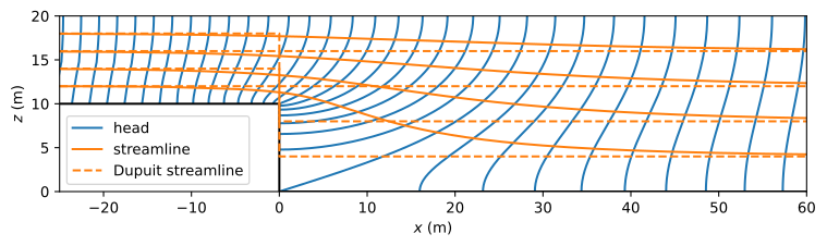
Figure 10.11 Flow net for confined flow with a jump in the base and vertical anisotropy \(k_x/k_z=10\); head contour interval \(\Delta h\)= 2 mm.

      The second example of vertical anisotropy is for the case that the vertical hydraulic conductivity is 100 times larger than the horizontal hydraulic conductivity. The much larger vertical than horizontal hydraulic conductivity approaches the Dupuit approximation (in which the vertical resistance to flow is completely neglected). The two solutions should thus be very similar. The flow net is shown in Figure 10.12; the code to produce the flow net is the same as for Figure 10.11 and is not repeated here. The head contours are indeed almost vertical, even near the jump in base, and the streamlines are horizontal and almost jump down vertically at the jump in the base.

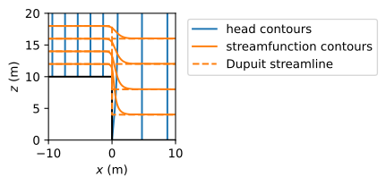
Figure 10.12 Flow net for confined flow with a jump in the base and vertical anisotropy \(k_z=100k_x\), which approaches the Dupuit approximation; head contour interval \(\Delta\)h= 2 mm.

Exercise 10.4

Compute the head drop between \(x=-50\) and \(x=50\) for the Dupuit solution and compute the additional head drop across the jump for the two-dimensional solution as compared to the Dupuit solution for the isotropic case.

Solution

Dupuit: \(\Delta h = 0.0750\, \mathrm{m}\), extra head drop: \(\Delta h = 0.0025\, \mathrm{m}\)