1.3. Areal recharge between an impermeable boundary and a river

The problem of the previous section is modified by replacing the river on the left side by an impermeable boundary (see Figure 1.11). The two boundary conditions become

(1.35)\[ \left. \frac{\text{d}h}{\text{d}x}\right\vert_{x=0} = 0 \]

(1.36)\[ h\vert_{x=L} = h_r \]

The boundary condition at \(x = L\) is referred to as a fixed-head or Dirichlet boundary condition. The boundary condition at \(x = 0\) is referred to as a specified-flux or Neumann boundary condition. The Dirichlet and Neumann boundary conditions are also referred to as type 1 and type 2 boundary conditions, respectively. In physical terms, the impermeable boundary can represent a water divide or a rock mass with very low permeability.

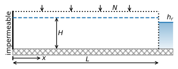
Figure 1.11 Areal recharge between an impermeable wall and a river.

      The general solution to the differential equation is again Eq. ((1.9)), of which the derivative with respect to \(x\) is

(1.37)\[ \frac{\text{d}h}{\text{d}x} = -\frac{N}{T}x + A \]

Application of boundary condition Eq. ((1.35)) at \(x = 0\) gives

(1.38)\[ A = 0 \]

so that application of boundary condition ((1.36)) leads to the following solution

(1.39)\[ h = -\frac{N}{2T}(x^2 - L^2) + h_r \]

and

(1.40)\[ Q_x = -T\frac{\text{d}h}{\text{d}x} = Nx \]

All the recharge flows to the river on the right, so the outflow into the right river is \(NL\). An example is provided below (Figure 1.12). Note that the line for the head function is horizontal at the left boundary, indicating the no-flow condition. The saturated thickness is approximated as constant and equal to \(H = 10\) m in the example below, but the distance between the head and the bottom of the aquifer (\(z_b\) = −5 m) varies from 14 m on the left side to 9 m on the right side. The question can be raised whether it is reasonable to approximate the saturated thickness as constant if it varies by this much. This question is addressed in Chapter 3.

# parameters
L = 1000 # aquifer length, m
H = 10 # aquifer thickness, m
zb = -5 # aquifer bottom, m
k = 10 # hydraulic conductivity, m/d
T = k * H # transmissivity, m^2/d
hr = 4 # specified head at the right boundary, m
N = 0.001  # areal recharge, m/d

# solution
x = np.linspace(0, L, 100)
h = -N / (2 * T) * (x ** 2 - L ** 2) + hr
Qx = N * x

# basic plot
plt.subplot(121)
plt.plot(x, h)
plt.subplot(122)
plt.plot(x, Qx);

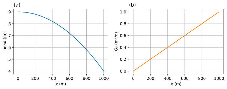
Figure 1.12 Areal recharge between an impermeable boundary and a river; head (left) and \(Q_x\) (right).

Exercise 1.7

Compute how long it takes for water that infiltrates at \(x = L/2\) to flow to the river. Use \(n = 0.3\).

Solution

\(t_\text{tr} = 2079\) d

Exercise 1.8

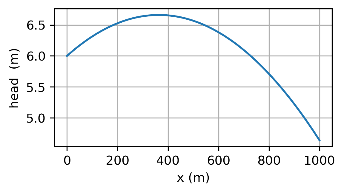
Derive and plot a solution for the head for the case that \(h\vert_{x=0} = h_l\) and \(\tfrac{\text{d}h}{\text{d}x}|_{x=L} = 0\), where \(h_l = 6\) m.

Solution

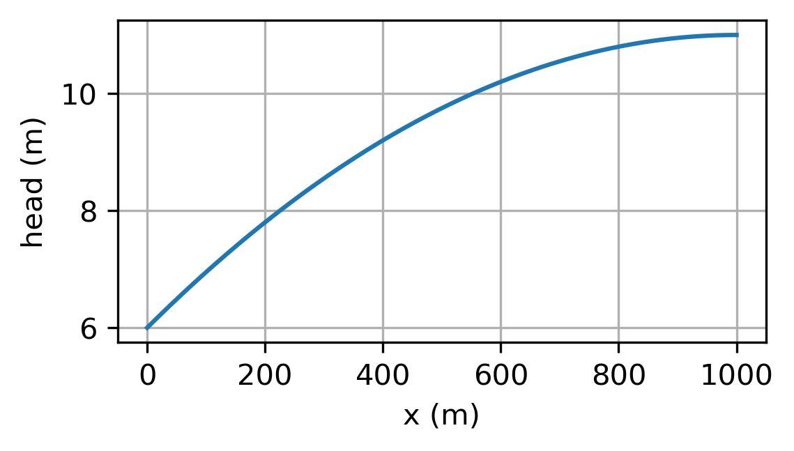
      Next, the boundary condition on the right side is modified by adding a layer with a resistance between the aquifer and the river (Figure 1.13). This resistance represents the low-permeable sediments that typically make up the river bed. In reality, the inflow occurs along the wet perimeter of the river, but to simplify the mathematical treatment, the leaky river bed is approximated here as a vertical section between the aquifer and the river with width \(w_h\) and horizontal hydraulic conductivity \(k_h\). The specific discharge through the layer is computed with Darcy’s law as

(1.41)\[ q_x = -k_h \frac{h_r - h_R}{w_h} = \frac{h_r - h_R}{c} \]

where \(h_r\) is the head in the aquifer at \(x=L\), \(h_R\) is the water level in the river, and \(c\) is referred to as the hydraulic resistance of the river bed and is defined as

(1.42)\[ c = \frac{w_h}{k_h} \]

Note that \(c\) has the dimension time. The discharge vector into the river is obtained through multiplication of \(q_x\) by the saturated thickness in the leaky layer, which is approximated here as \(H\).

(1.43)\[ Q_x\vert_{x=L} = H\frac{h_r-h_R}{c} = C(h_r - h_R) \]

where \(C=H/c\) is called the river bed conductance. This boundary condition represents a relation between the head and the flow and is referred to as a Robin boundary condition or a type 3 boundary condition.

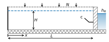
Figure 1.13 Areal recharge between an impermeable boundary and a river with river bed resistance.

      For this modified problem, the flow into the river is known upfront from continuity of flow and is equal to the total recharge \(NL\) so that

(1.44)\[ Q_x\vert_{x=L} = C(h_r-h_R)=NL \]

and the head in the aquifer at \(x=L\) is

(1.45)\[ h_r=\frac{NL}{C} + h_R \]

The solution for the head and flux can now be obtained from Eqs. ((1.39)) and ((1.40)). The shape of the head curve is the same as for the case without entry resistance (Figure 1.12), but all heads are raised by an amount \(NL/C\) (Figure 1.14), because all the water needs to flow through the resistance layer into the river. For the parameters of the previous example, but with an entry resistance of \(c = 10\) d, the head increase is 1 m.

# additional parameters
hR = 4 # water level in river, m
c = 10 # hydraulic resistance of river bed, d

# solution
x = np.linspace(0, L, 100)
C = H / c
hr = N * L / C + hR
h = -N / (2 * T) * (x ** 2 - L ** 2) + hr
Qx = N * x

# basic plot
plt.subplot(121)
plt.plot(x, h)
plt.subplot(122)
plt.plot(x, Qx);

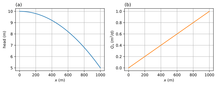
Figure 1.14 Areal recharge between an impermeable wall and a river with riverbed resistance; head (left) and \(Q_x\) (right).

Exercise 1.9

Compute the head in the aquifer at \(x = L\) for the case with river bed conductance, but now the boundary condition on the left side is \(h\vert_{x=0}=6\). Plot the head vs. \(x\).

Solution

\(h_r = 4.64\) m