8.1. Uniform flow and wells

In this section, an analytic element code is developed to simulate wells, uniform flow, and a constant. The discharge potential is written as

(8.1)\[ \Phi = \sum_{m=1}^{M} \frac{Q_m}{2\pi}\ln(r_m) + \sum_{n=1}^{N} \frac{P_n}{2\pi}\ln(r_n) -Q_u(x\cos(\theta) + y\sin(\theta)) + C \]

where \(M\) is the number of wells with a specified discharge \(Q_m\), \(N\) is the number of wells with a head-specified condition, and \(P_n\) is the discharge of head-specified well \(n\), which is unknown upfront; \(Q_u\) is the magnitude of the uniform flow (the parameter) and \(\theta\) is the direction of uniform flow; the constant \(C\) is also a priori unknown and is computed from a specified-head condition. The transmissivity is approximated as constant throughout the model.
     The analytic element code is developed using object oriented programming; an introduction to object oriented programming for Python may be found in, e.g., Lutz (2013). The analytic element code consists of a Model class and a number of Element classes. The Model class stores the transmissivity of the aquifer and a Python list called elements that contains all the elements in the model; the element list is initially empty. The Model class has a potential function to compute the discharge potential at a point caused by all analytic elements in the model (Eq. (8.1)). In addition, the Model class has a head function to compute the head at a point; the head function internally calls the potential function and then converts the potential to a head. Finally, the Model class has a solve method, which computes the parameters of all head-specified elements in the model. This function is included here, but will be explained later on.

class Model:
    
    def __init__(self, T):
        self.T = T
        self.elements = [] # list of all elements
        
    def potential(self, x, y):
        pot = 0.0
        for e in self.elements:
            pot += e.potential(x, y)
        return pot
        
    def head(self, x, y):
        return self.potential(x, y) / self.T
    
    def solve(self):
        esolve = [e for e in self.elements if e.nunknowns == 1]
        nunknowns = len(esolve)
        matrix = np.zeros((nunknowns, nunknowns))
        rhs = np.zeros(nunknowns)
        for irow in range(nunknowns):
            matrix[irow], rhs[irow] = esolve[irow].equation()
        solution = np.linalg.solve(matrix, rhs)
        for irow in range(nunknowns):
            esolve[irow].parameter = solution[irow]

     The Element class is the base class of all analytic elements. It stores the model that the element is added to, the value of the parameter (e.g., the discharge of a well), the number of unknown parameters of an element, which is zero by default, and it adds the element to the specified model by adding it to the elements list of the model. The Element class includes the potential function, which is the same for all elements. The potential function computes the discharge potential of an element by returning the product of the influence function potinf of the element and the parameter of the element. Every element must implement its own potential influence function potinf, which is the discharge potential for the case that the parameter of the element equals one. The utility of influence functions will become apparent further on in this section, when elements are introduced that have an a priori unknown parameter, for example a well where the discharge is unknown and is computed from a specified head at the well.

class Element:
    
    def __init__(self, model, p):
        self.model = model
        self.parameter = p
        self.nunknowns = 0
        self.model.elements.append(self)
        
    def potential(self, x, y):
        return self.parameter * self.potinf(x, y)
    
    def potinf(self, x, y):
        pass

     Every element is derived from the Element base class, so that it automatically gets all attributes and functions from the Element class. The Well class, for wells with a specified discharge, takes as input arguments the model to which the well is added, the location \((x_w,y_w)\) of the well, the discharge of the well, and the radius of the well. The Well class is derived from the Element class, which stores the parameter (the discharge). The Well class stores the location and the radius of the well. Only one function needs to be implemented for the Well class: the potinf function, which for a well is

(8.2)\[ \Phi = \frac{1}{2\pi}\ln(r) \]

where \(r=\sqrt{(x-x_w)^2 + (y-y_w)^2}\) is the radial distance between the well and point \((x,y)\). The radial distance is set to the radius of the well for points inside the radius of the well using the np.where function.

class Well(Element):
    
    def __init__(self, model, xw=0, yw=0, Q=1, rw=0.3):
        Element.__init__(self, model, p=Q)
        self.xw, self.yw = xw, yw
        self.rw = rw
            
    def potinf(self, x, y):
        r = np.sqrt((x - self.xw)**2 + (y - self.yw)**2)
        r = np.where(r < self.rw, self.rw, r)
        return 1 / (2 * np.pi) * np.log(r)

     The UniformFlow class is also derived from the Element class and takes as input arguments the model to which it is added, the absolute value of the head gradient, and the direction \(\theta\) of uniform flow (in degrees measured counter-clockwise from the positive \(x\)-direction). The potinf function is

(8.3)\[ \Phi = -Q_u(x\cos(\theta) + y\sin(\theta)) \]

where the magnitiude \(Q_u\) is computed as the product of the transmissivity and the absolute value of the gradient.

class UniformFlow(Element):
    
    def __init__(self, model, gradient, angle):
        Element.__init__(self, model, p=model.T * gradient)
        self.theta = np.deg2rad(angle)
        
    def potinf(self, x, y):
        return -(x * np.cos(self.theta) + y * np.sin(self.theta))

      An analytic element model may now be constructed by creating a Model object, and optionally adding a uniform flow object and an arbitrary number of wells. The head and potential may be computed at any point. In the example below, one extraction well and one injection well are situated in an otherwise uniform flow field in the southeastern direction \((\theta=-45^\circ)\). Equipotentials are plotted in Figure 8.1. Note that the magnitude of the discharge of the extraction well is twice as large as for the injection well.

# parameters and model
ml = Model(T=100) # transmissivity, m^2/d
Well(ml, xw=50, yw=0, Q=200) # extraction well, Q in m^3/d
Well(ml, xw=0, yw=0, Q=-100) # injection well, Q in m^3/d
UniformFlow(ml, gradient=0.002, angle=-45);

# solution
xg, yg = np.meshgrid(np.linspace(-100, 100, 100), np.linspace(-75, 75, 100))
pot = ml.potential(xg, yg)

# basic equipotentials plot
plt.subplot(111, aspect=1)
plt.contour(xg, yg, pot, 20)

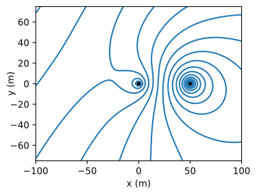
Figure 8.1 Equipotentials for analytic element model of an injection well (\(Q=-100\) m\(^3\)/d) and an extraction well (\(Q=200\) m\(^3\)/d) in uniform flow in southeastern direction.

Exercise 8.1

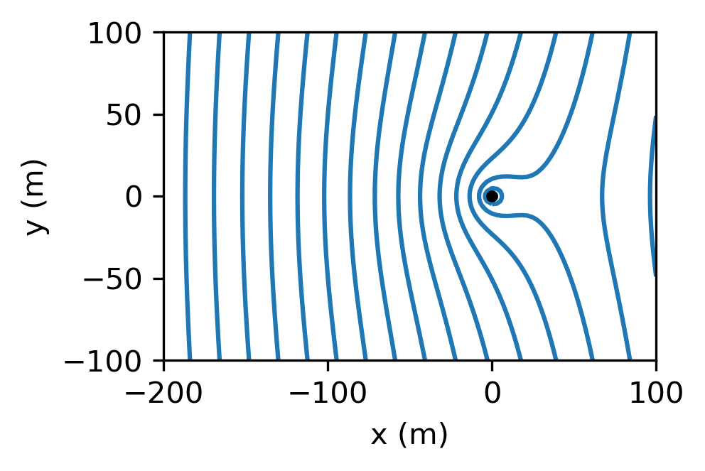
Create equipotentials for the example in Section 7.1 of a well in uniform flow using (like the left graph of Figure 7.1) using the analytic element code developed above. Use a transmissivity of \(T=250\) m\(^2\)/d.

Solution

     The head must be defined at at least one point in the aquifer, otherwise the head values along the contours are meaningless (an arbitrary value can be added to all values, resulting in the same flow field). Two types of head-specified elements are implemented in this section: wells with a specified head and an additive constant which is also computed from a specified-head condition. The free parameters of head-specified elements are computed by building a system of equations for all head-specified conditions and solving for all free parameters simultaneously. This procedure is illustrated by solving a problem with uniform flow, two wells, and a constant.
     Consider an aquifer with uniform flow \(U\) in the positive \(x\)-direction with two wells and a real constant \(C\) (see Figure 8.2). Well 0 is located at \((x,y)=(0,0)\) and has a specified discharge \(Q\). Well 1 is located at \((x,y)=(a,b)\) and has a discharge \(P\). The radius of both wells is \(r_w\). The potential for this problem is obtained from superposition of the potential of uniform flow ((7.1)), the potentials for two wells ((6.37)), and a constant \(C\):

(8.4)\[ \Omega = -Ux + \frac{Q}{2\pi}\ln(r_0) + \frac{P}{2\pi}\ln(r_1) + C \]

where \(r_0\) and \(r_1\) are the distances from wells 0 and 1, respectively. The discharge discharge \(P\) is unknown and must be computed such that the head equals \(h_w\) at well 1. Furthermore, the head at \((x,y)=(a,0)\) is known to be \(h_0\). This gives two equations for the two unknown parameters \(C\) and \(P\).
     The parameters \(P\) and \(C\) are obtained from the system of two linear equations

(8.5)\[\begin{split} \begin{split} &\Phi|_{x=a,y=0} = \Phi_0 \\ &\Phi|_{x=a+r_w,y=b} = \Phi_w \end{split} \end{split}\]

where \(\Phi_0\) and \(\Phi_w\) are the potential equivalents of \(h_0\) and \(h_w\), respectively. Note that the head at well 1 is specified at \((x,y)=(a+r_w, b)\) which is referred to as the collocation point; specification at another point on the well screen may result in a slightly different solution, but the difference is commonly negligible. Substitution of ((8.4)) for \(\Phi\) in ((8.5)) and rearrangement of terms gives the following system of two equations in two unknowns

(8.6)\[\begin{split} \begin{split} \frac{P}{2\pi}\ln(b) + C &= \Phi_0 + Ua- \frac{Q}{2\pi}\ln(a) \\ \frac{P}{2\pi}\ln(r_w) + C &= \Phi_w + U(a + r_w) - \frac{Q}{2\pi}\ln(d) \end{split} \end{split}\]

where \(d=\sqrt{(a + r_w)^2 + b^2}\) is the distance between the well with specified discharge and the collocation point on the well screen of the head-specified well. In matrix form, the system of equations is

(8.7)\[\begin{split} \begin{pmatrix} \frac{1}{2\pi}\ln(b) & 1 \\ \frac{1}{2\pi}\ln(r_{w}) & 1 \\ \end{pmatrix} \begin{pmatrix} P \\ C \end{pmatrix} = \begin{pmatrix} \Phi_0 + U a - \frac{Q}{2\pi}\ln(a)\\ \Phi_w + U(a + r_w) - \frac{Q}{2\pi}\ln(d) \end{pmatrix} \end{split}\]

The unknown free parameters \(P\) and \(C\) are obtained by solving this system of two linear equations.
     The solve method of the Model class, as defined above, counts the number of elements with an unknown parameter and stores them in a separate list called esolve, builds the matrix and the right-hand side of the system of equations, solves the system, and stores the computed parameters for the corresponding head-specified elements (in this case the values of \(P\) and \(C\)). The solve method loops through all elements in the esolve list and calls their equation function, which returns one row for the matrix and one right-hand side value. The equation method of the Constant element (not yet defined) returns the first row of the matrix and the first value of the right-hand side vector, and the equation method of well 1 (the head-specified well) returns the second row of the matrix and the second value of the right-hand side vector.
     The equation function is stored in a separate mix-in class HeadEquation, as it is the same for all head-specified elements. Each element that uses this mix-in class must store the location of the collocation point where the head is specified as xc and yc, and the specified value of the discharge potential at the collocation point as pc. The equation function starts out with a row of the matrix that is an empty list and a right-hand side value that is equal to the specified discharge potential pc. The equation function then loops through all the elements in the model. If an element has an unknown parameter (nunkonwns==1), its potential influence function potinf is evaluated at the collocation point and is stored as the next value in the row of the matrix. If an element does not have an unknown parameter, its potential function is evaluated at the collocation point and the returned value is subtracted from the right-hand side value.

class HeadEquation:

    def equation(self):
        row = []
        rhs = self.pc
        for e in self.model.elements:
            if e.nunknowns == 1:
                row.append(e.potinf(self.xc, self.yc))
            else:
                rhs -= e.potential(self.xc, self.yc)
        return row, rhs

      The HeadWell class for head-specified wells can now be derived from both the Well class and the HeadEquation class. Input arguments are the model to which the element is added, the location of the well, the radius, and the specified head. The xc and yc locations of the collocation point are stored, as well as the specified potential pc at the collocation point. The number of unknowns parameters nunknowns is set to 1. All other attributes and functions are inherited from the Well and HeadEquation classes.

class HeadWell(Well, HeadEquation):
    
    def __init__(self, model, xw, yw, rw, hw):
        Well.__init__(self, model, xw, yw, 0, rw)
        self.xc, self.yc = xw + rw, yw
        self.pc = self.model.T * hw
        self.nunknowns = 1

      The Constant class is derived from the Element class and the HeadEquation class. Input arguments are the model to which the element is added and the location and value of the specified head. The potinf function of the Constant class is simply equal to 1. The Constant element is also referred to as the reference point.

class Constant(Element, HeadEquation):
    
    def __init__(self, model, xc, yc, hc):
        Element.__init__(self, model, p=0)
        self.xc, self.yc = xc, yc
        self.pc = self.model.T * hc
        self.nunknowns = 1
        
    def potinf(self, x, y):
        return np.ones_like(x, dtype='float')

     The example problem of Figure 8.2 (as discussed above) is solved with the analytic element code developed so far. The analytic element model is created with the following five commands

# parameters and model
ml = Model(T=100) # transmissivity in m^2/d
w1 = Well(ml, xw=0, yw=0, Q=100, rw=0.3) # Q in m^3/d
w2 = HeadWell(ml, xw=400, yw=300, rw=0.3, hw=20)
uf = UniformFlow(ml, gradient=0.002, angle=0)
rf = Constant(ml, xc=400, yc=0, hc=22)

      In the code cell above, the model object is stored in the variable ml. The unknown parameters in the model may be computed by calling the solve method of the model. The head at the head-specified well and at the reference point are computed to verify that the solution is indeed correct. In addition, the head at the discharge-specified well and the computed discharge of the head-specified well are printed to the screen. A grid of the head is computed and the minimum and maximum values on the grid are printed to the screen, which are used to specify values for the contours to be plotted. Finally, head contours are plotted (right graph in Figure 8.2).

# solution
ml.solve() # compute the unkown parameters
print(f'computed head at discharge-specified well: {ml.head(0, 0):.2f} m')
print(f'computed head at head-specified well: {ml.head(400.3, 300):.2f} m')
print(f'computed discharge of head-specified well: {w2.parameter:.2f} m^3/d')
print(f'computed head at reference point: {ml.head(400, 0):.2f} m')
# grid
xg, yg = np.meshgrid(np.linspace(-200, 600, 100), np.linspace(-100, 500, 100))
head = ml.head(xg, yg)
print(f'min and max head on grid: {head.min():.2f}, {head.max():.2f}')

computed head at discharge-specified well: 21.81 m
computed head at head-specified well: 20.00 m
computed discharge of head-specified well: 185.10 m^3/d
computed head at reference point: 22.00 m
min and max head on grid: 20.57, 23.47

# basic head contours (right graph)
plt.subplot(111, aspect=1)
plt.contour(xg, yg, head, np.arange(20, 24, 0.2));

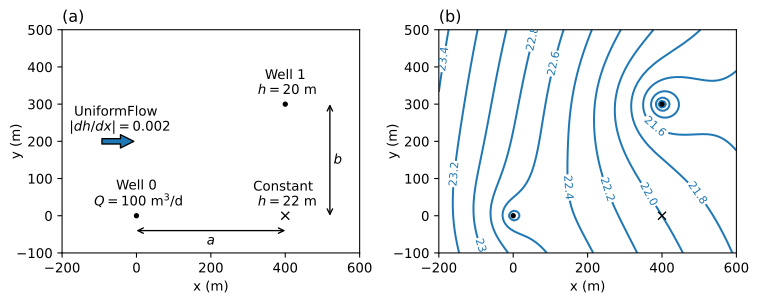
Figure 8.2 Layout of analytic element model (left) and corresponding head contours (right).

Exercise 8.2

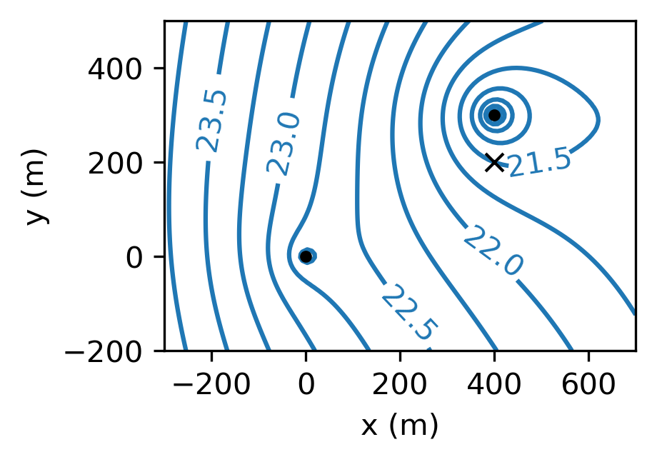
Modify the HeadWell class to specify an optional location of the control point. Plot head contours for the previous example, but now the head for the head-specified well is 21.5 m and is specified at \((x,y)=(400,200)\). Compute the head at the head-specified well and the discharge of the head-specified well.

Solution

\(h = 18.8\) m, \(Q = 296\) m\(^3\)/d

An interactive figure of the head contours is added for the example of Figure 8.1, where a reference point with a head of 20 m is added at \((x,y)=(25, 70)\).

Figure 8.3 Head contours for two wells in uniform flow. The red contour is for \(h=20\) m and goes through the reference point (black cross). Contour interval is 10 cm.