10.1. Vertical anisotropy

The hydraulic conductivity is often anisotropic, where the vertical component of the hydraulic conductivity is smaller than the horizontal component. One of the main reasons for vertical anisotropy is that aquifers often consist of alternating layers of somewhat coarser and somewhat finer material. The average value of the hydraulic conductivity in the horizontal direction is dictated by the hydraulic conductivity of the coarser layers, while the average value in the vertical direction is dictated by the hydraulic conductivity of the finer layers. In practice, it is popular to use an anisotropy factor of 10 (the vertical hydraulic conductivity is 10 times smaller than the horizontal hydraulic conductivity), but a good reason for this number does not exist. For the case that the hydraulic conductivity is anisotropic with \(k_x\) in the \(x\)-direction and \(k_z\) in the \(z\)-direction, Darcy’s law becomes

(10.7)\[ q_x = -k_x\frac{\partial h}{\partial x} {\hskip 2em} q_z = -k_z\frac{\partial h}{\partial z} \]

Substitution of these equations for \(q_x\) and \(q_z\) in the continuity equation ((10.1)) gives

(10.8)\[ \frac{\partial}{\partial x}\left(k_x \frac{\partial h}{\partial x}\right) + \frac{\partial}{\partial z}\left(k_z \frac{\partial h}{\partial z}\right)= 0 \]

This equation may be transformed into Laplace’s equation by a change of variables

(10.9)\[ \tilde{x} = x\sqrt{k_z/k_x} {\hskip 2em} \tilde{z} = z \]

which gives

(10.10)\[ \frac{\partial^2 h}{\partial \tilde{x}^2} + \frac{\partial^2 h}{\partial \tilde{z}^2} = 0 \]

Hence, in the \(\tilde{x}, \tilde{z}\) domain, the head is governed by Laplace’s equation. The specific discharge in the transformed domain can be evaluated with Darcy’s law using the isotropic hydraulic conductivity \(\tilde{k}\) defined as

(10.11)\[ \tilde{k} = \sqrt{k_xk_z} \]

The use of \(\tilde{k}\) ensures that the net discharge in the isotropic transformed domain is the same as the net discharge in the original anisotropic domain. For example, the net flux \(Q_\text{net}\) across a small section \(\Delta z\) in the anisotropic domain equals

(10.12)\[ Q_\text{net} = -k_x \frac{\partial h}{\partial x} \Delta z \]

and is equal to the net flux across the same section in the transformed isotropic domain

(10.13)\[ \tilde{Q}_\text{net} = -\tilde{k}\frac{\partial h}{\partial \tilde{x}} \Delta \tilde{z}= -\sqrt{k_xk_z}\frac{\partial h}{\partial x} \frac{1}{\sqrt{k_z/k_x}} \Delta z = -k_x \frac{\partial h}{\partial x} \Delta z = Q_\text{net} \]

The same holds in the \(z\)-direction.
      In summary, an anisotropic problem may be solved with standard methods for Laplace’s equation, provided that the \(x\) direction of the flow field is squeezed according to Eq. ((10.9)), and the isotropic hydraulic conductivity (Eq. (10.11)) is used in the transformed domain. A complex specific discharge potential in the transformed potential may be defined as \(\tilde{\omega}=\tilde{\phi} + i\tilde{\psi}\), where \(\phi=\tilde{k}h\) and \(\tilde{\psi} = \psi\).
      As a simple example, consider a rectangular domain with length \(L\) and height \(B\) (Figure 10.1). The head at the origin in the lower left-hand corner equals zero. Flow is uniform, and the head gradients in the \(x\)- and \(z\)-directions are equal: \(\partial h/\partial x= \partial h / \partial z = a\). As such, the head varies linearly along the boundaries (Figure 10.1). The hydraulic conductivities in the \(x\) and \(z\) directions are \(k_x\) and \(k_z\), respectively.
      The flow is uniform in both the anisotropic physical domain and the isotropic transformed domain. In the physical domain, \(q_x=-k_xa\) and \(q_z=-k_za\). In the transformed domain, \(\tilde{q}_x\) and \(\tilde{q}_z\) are

(10.14)\[ \tilde{q}_x = -\tilde{k}\frac{\partial h}{\partial \tilde{x}} = -\tilde{k}\frac{\partial h}{\partial x}\frac{\partial x}{\partial \tilde{x}} = -\frac{\tilde{k}a}{\sqrt{k_z/k_x}} \]

(10.15)\[ \tilde{q}_z=-\tilde{k}a \]

The solution for the complex specific discharge potential in the transformed domain is (see Section 7.3)

(10.16)\[ \tilde{\omega} = -(\tilde{q}_x- \tilde{q}_zi) \tilde{\zeta} \]

where \(\tilde{\zeta}=\tilde{x} + i\tilde{z}\) is the complex coordinate in the transformed domain.
      An example flow field is shown below in Figure 10.1. The flow field is shown in both the transformed domain and in the problem domain. Note that the streamlines and head contours intersect at right angles in the transformed domain, where the hydraulic conductivity \(\tilde{k}\) is isotropic, but don’t intersect at right angles in the problem domain where the hydraulic conductivity is anisotropic.

# parameters
L = 1000 # length of domain, m
B = 300 # width of domain, m
kx = 5 # hydraulic conductivity in x-direction, m/d
kz = 1 # hydraulic conductivity in z-direction, m/d
a = -0.002 # head gradient in x and z directions

# solution
kt = np.sqrt(kx * kz)
qxt = -kt * a / np.sqrt(kz / kx)
qzt = -kt * a
xg, zg = np.meshgrid(np.linspace(0, L, 10), np.linspace(0, B, 10))
xt = xg * np.sqrt(kz / kx)
zt = zg
zetat = xt + 1j * zt
omt = -(qxt - 1j * qzt) * zetat
h = omt.real / kt
psi = omt.imag

# basic flow net
plt.subplot(121, aspect=1) # problem domain
plt.contour(xg, zg, h, 10)
plt.contour(xg, zg, psi, 10);
plt.subplot(122, aspect=1) # transformed domain
plt.contour(xt, zt, h, 20)
plt.contour(xt, zt, psi, 20);

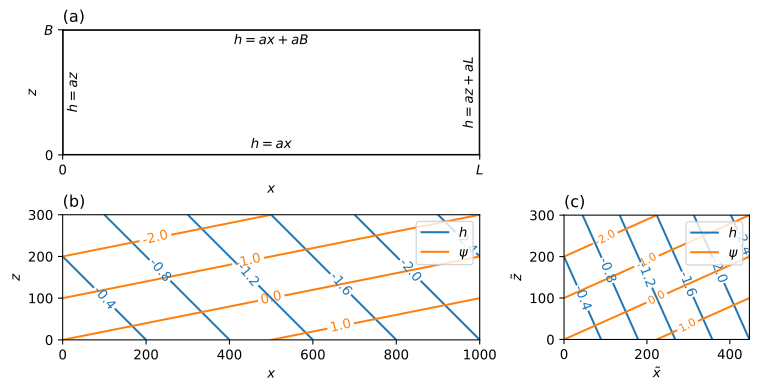
Figure 10.1 Example for uniform flow in an anisotropic aquifer; boundary conditions (upper left), flow net in squeezed transformed domain (lower right), and flow net in problem domain (lower left).