10.5. Interface flow towards the coast

Several solutions for interface flow in coastal aquifers were discussed in this book so far (Chapter 4 and Section 7.4), all based on the Dupuit approximation. The width of the outflow zone at the coast was zero for all presented Dupuit solutions, except for the solution with a resistance layer along the sea bottom (Section 4.3). In Chapter 4, it was claimed that the resulting interface was, nevertheless, a good approximation, even though flow near the coast has a significant vertical component. In this and the following section, Dupuit solutions are compared to solutions for two-dimensional flow in the vertical plane, and it is investigated how wide the outflow zone below the sea is.
      Consider steady two-dimensional interface flow in the vertical plane in a confined coastal aquifer. The aquifer is so deep that the interface does not reach the bottom of the aquifer; the saltwater is at rest (Figure 10.17). The density of the freshwater is \(\rho_f\), the density of the saltwater is \(\rho_s\), and the hydraulic conductivity of the aquifer is isotropic and equal to \(k\). The sea bottom is horizontal and at the same elevation as the top of the confined aquifer. The origin of the coordinate system is chosen at the coastline at the top of the aquifer. Flow towards the coast is constant and equal to \(Q_x=U\). The stream function along the top of the aquifer is chosen to equal \(\psi=0\), so that the stream function along the interface equals \(\psi=U\).
      This problem is known as a free boundary problem. The location of the interface is a free boundary because it is unknown prior to solving the problem. There are two conditions specified along the interface: the interface is an impermeable boundary and the elevation of the interface \(z_i\) is related to the head \(h_i\) along the interface according to the Ghyben-Herzberg equation (Chapter 4)

(10.48)\[ z_i = -\alpha h_i \]

where

(10.49)\[ \alpha = \frac{\rho_f}{\rho_s - \rho_f} \]

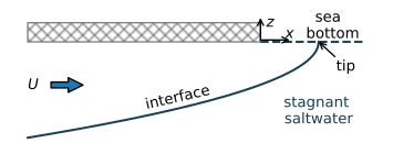
Figure 10.17 Interface flow towards the coast.

      The stated problem is known as Glover’s problem (Glover, 1959). The complex potential solution used here is obtained from Bruggeman (Bruggeman 1999, Eq. 910.01), as

(10.50)\[ \omega = \sqrt{-2 k U \zeta / \alpha} \]

where \(\zeta=x + iz\) is the complex coordinate. The solution for the complex potential can be inverted, which gives

(10.51)\[ \zeta = \frac{-\omega^2 \alpha}{2k U} \]

The specific discharge potential along the interface equals \(\phi_i=-k z_i / \alpha\) and the stream function is equal to the stream function along the bottom of the aquifer (\(\psi=U\)). An equation for the elevation of the interface as a function of \(x\) may be obtained by substituting \(\omega=-k\alpha z_i + Ui\) for \(\omega\) and \(x+iz_i\) for \(\zeta\) in ((10.50)), which gives, after some algebra

(10.52)\[ z_i = -\sqrt{\frac{U^2\alpha^2}{k^2} - \frac{2U\alpha x}{k}} \]

The tip of the interface is the point where the interface intersects the sea bottom (Figure 10.17). The location of the tip of the interface \(x_\text{tip}\) is obtained by setting \(z_i=0\) in Eq. ((10.52)) and solving for \(x\), which gives

(10.53)\[ x_\text{tip} = \frac{U\alpha}{2k} \]

This means that the outflow zone is wider for a larger value of the flow towards the coast \(U\).
      In the example below, a flow net is computed by specifically computing the locations of the streamlines and equipotentials, as \(\zeta\) is known as a function of \(\omega\) (Eq. (10.51)) . For the chosen parameters, the interface is already 7 m deep at a distance of 14 m inland from the coastline (Figure 10.18). The length of the outflow face is just 0.8 m.

# parameters
k = 10 # hydraulic conductivity, m/d
rhof = 1000 # density freshwater, kg/m^3
rhos = 1025 # density of saltwater, kg/m^3
U = 0.4 # flow towards the coast, m^2/d

# solution
alpha = rhof / (rhos - rhof)
n = 100
zeta_streamlines = []
zeta_equipotentials = []
for psi in np.linspace(0, U, 6):
    omega = np.linspace(0, 2, n) + 1j * psi
    zeta = -omega**2 * alpha / (2 * k * U)
    zeta_streamlines.append(zeta)
for phi in np.arange(0, 2, U / 6):
    omega = phi + 1j * np.linspace(0, U, n)
    zeta = -omega**2 * alpha / (2 * k * U)
    zeta_equipotentials.append(zeta)
zetatip = -(1j * U) ** 2 * alpha / (2 * k * U)
print(f'location of the tip: {zetatip.real: .2f} m')

location of the tip:  0.80 m

# basic plot
plt.subplot(111, aspect=1, xlim=(-15, 1))
for zeta in zeta_equipotentials:
    plt.plot(zeta.real, zeta.imag, 'C0')
for zeta in zeta_streamlines:
    plt.plot(zeta.real, zeta.imag, 'C1')

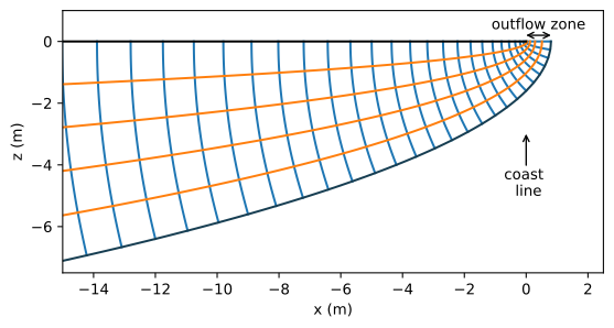
Figure 10.18 Flow net for two-dimensional flow of fresh water towards the coast (Glover’s solution).

      The interface position obtained with Glover’s solution is compared to a Dupuit interface solution. The Dupuit solution for the elevation of the interface is obtained from Section 4.1 as

(10.54)\[ z_i = -\sqrt{\frac{-2U \alpha x}{k}} \]

Note that \(z_i^2\) of the two-dimensional solution ((10.52)) differs by a constant factor from the Dupuit solution. The difference between the Glover solution and the Dupuit solution is minor for the parameters of the example (Figure 10.19).
      The difference between the two solutions becomes a bit larger when the vertical hydraulic conductivity \(k_z\) of the aquifer is significantly smaller than the horizontal hydraulic conductivity \(k_x\). The Glover solution is modified for an anistropic hydraulic conductivity using the approach of Section 10.1. The solution for the complex potential is

(10.55)\[ \tilde{\omega} = \sqrt{-2 \tilde{k} U \tilde{\zeta} / \alpha} \]

The corresponding elevation of the interface is

(10.56)\[ z_i = -\sqrt{\frac{U^2\alpha^2}{k_x k_z} - \frac{2U\alpha x}{k_x}} \]

and the location of the tip of the interface is

(10.57)\[ x_\text{tip} = \frac{U\alpha}{2k_z} \]

In the example below, the interface is plotted for the isotropic case and for the case that \(k_z=k_x/10\), which results in an outflow zone that is 10 times wider than for the isotropic case (Figure 10.19). The interface is located somewhat deeper than for the isotropic case. The Dupuit solution does not change, of course, as the resistance to flow in the vertical direction is neglected.
      The Dupuit solution is a very good approximation of the isotropic Glover solution and a reasonable approximation of the anisotropic Glover solution. The Dupuit solution is always conservative when assessing the extent of seawater intrusion: the thickness of the freshwater zone is always smaller and the seawater intrusion more severe than in the Glover solution. The largest difference in the thickness of the freshwater zone is at the coastline.

# additional parameters anisotropic case
kx = k
kz = k / 10

# isotropic solution
xtip = U * alpha / (2 * k)
xglover = np.linspace(-150, xtip, 100)
zglover = -np.sqrt(U * alpha / k * (U * alpha / k - 2 * xglover))
# aniosotropic solution
xtipaniso = U * alpha / (2 * kz)
xaniso = np.linspace(-150, xtipaniso, 200)
zaniso = -np.sqrt(U * alpha / kx * (U * alpha / kz - 2 * xaniso))
print(f'location of the tip for anisotropic case: {xtipaniso: 0.2f} m')
#
xdupuit = np.linspace(-150, 0, 100)
zdupuit = -np.sqrt(-2 * U * alpha * xdupuit / k)

location of the tip for anisotropic case:  8.00 m

# basic plot (Fig. 10.15)
plt.plot(xglover, zglover, 'C1', label='Glover $k_z=k_x$')
plt.plot(xaniso, zaniso, 'C2', label='Glover $k_z=k_x/10$')
plt.plot(xdupuit, zdupuit, 'C1--', label='Dupuit $H=20$')
plt.legend();

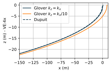
Figure 10.19 Comparison of interface elevation between the Glover solution (both isotropic and anisotropic) and the Dupuit solution.

Exercise 10.7

Compute the ratio of the depth of the interface and the head at the interface at \(x=-50\) and at \(x=-100\) for the anisotropic case (Hint: the answer is of course \(\alpha\) if you do this correctly). Next, compute the ratio of the depth of the interface and the head at the top of the aquifer at \(x=-50\) and at \(x=-100\) for the anisotropic case.

Solution

Factor based on head at the top of aquifer at \(x = −100\) m: \(41.6\).
Factor based on head at the top of aquifer at \(x =−50\) m: \(43.1\)