9.1. Wells in confined and unconfined aquifers

In this section, a solution is presented for transient flow to a well in an aquifer with constant transmissivity \(T\) and storage coefficient \(S\). The governing differential equation is ((9.5)). The well starts pumping with discharge \(Q\) at time \(t = t_0\). The boundary condition at the well is approximated as (similar to boundary condition ((6.24)))

(9.6)\[ \lim_{r \to 0} -2\pi r Q_r = Q {\hskip 2em} t\ge t_0 \]

Initially, the head change in the aquifer caused by the transient well is, of course, equal to zero

(9.7)\[ h|_{r, t=t_0} = 0 \]

The second boundary condition is that the head change caused by the well at infinity is zero at all time

(9.8)\[ h|_{r=\infty, t} = 0 \]

The solution for the head is a function of the radial distance, \(r\), from the well and time and is known as the Theis solution (Theis, 1935)

(9.9)\[ h = - \frac{Q}{4\pi T}\text{E}_1\left( u\right) {\hskip 2em} t\ge t_0 \]

where

(9.10)\[ u = \frac{S r^2}{4T(t-t_0)} \]

and E\(_1\) is the exponential integral defined as

(9.11)\[ \text{E}_1(u) = \int_u^{\infty} \frac{\exp(-s)}{s}d s \]

      The head starts to decrease after the well starts pumping. The drop in head is also referred to as the drawdown. So a drawdown of, e.g., 1 m means that \(h = −1\) m. The head is a function only of the dimensionless parameter \(u\). Hence, if a certain drawdown is reached at a distance \(r_1\) after a time period \(\Delta t_1\) of pumping, the same drawdown is reached at a distance \(2r_1\) after a time period \(4\Delta t_1\) of pumping, as both combinations of time and radial distance result in the same value of \(u\)

(9.12)\[ u = \frac{S r_1^2}{4T\Delta t_1} = \frac{S (2r_1)^2}{4T(4 \Delta t_1)} \]

      The function E\(_1\) is available as exp1 from the scipy.special package, but there also exists a series representation, which is useful for the evaluation of limiting cases (e.g., large time). The series representation is (e.g., Abramowitz and Stegun, 1965)

(9.13)\[ \text{E}_1(u) = -\gamma -\ln u - \sum_{n=1}^\infty \frac{ (-u)^n}{n\cdot n!} \]

where \(\gamma=0.5772...\) is Euler’s constant, available from numpy as euler_gamma. The series for E\(_1\) converges quickly when \(u<1\). Only the first two terms are needed when \(u\) is small, in which case the formula for the head may be approximated as

(9.14)\[ h \approx \frac{Q}{4\pi T}\left[\gamma + \ln\left(\frac{S r^2}{4T(t-t_0)}\right)\right] {\hskip 2em} u < 0.1 \]

Note that \(u\) is small when \(r\) is small or when \(t\) is large, or both.
      The head inside the well is computed by evaluating the Theis solution at the well radius \(r_w\). Four curves are shown in the graphs of Figure 9.1: the head \(h_w\) inside the well, the head \(h_{20}\) at \(r = 20\) m, the difference \(h_w-h_{20}\), and the head \(h_{20}\) computed with the approximate formula ((9.14)). The time axis is linear in the left graph and log-scaled in the right graph. The difference \(h_w-h_{20}\) becomes constant after ∼0.01 d for this case. The approximate formula results in a straight line in the graph with a log-scaled time axis, as can also be seen from Eq. ((9.14)). The approximate formula gives good results for \(u < 0.1\), which corresponds to \(t > 0.01\) d for this case and at this location.

# parameters
T = 200 # transmissivity, m^2/d
S = 2E-3 # storage coefficient, -
rw = 0.3 # radius of well, m
Q = 1000 # discharge of well, m^3/d
t0 = 0 # start of pumping, d
r = 20 # location of h20, m

# solution
from scipy.special import exp1
def htheis(r, t, T, S, Q, t0=0):
    return -Q / (4 * np.pi * T) * exp1(S * r ** 2 / (4 * T * (t - t0)))

t = np.logspace(-3, 0, 100)
hw = htheis(rw, t, T, S, Q, t0)
h20 = htheis(20, t, T, S, Q, t0)
h20approx = Q / (4 * np.pi * T) * (np.euler_gamma + 
                                   np.log(S * r ** 2 / (4 * T * (t - t0))))

# basic plot
plt.subplot(121)
plt.plot(t, hw, label='$h_w$')
plt.plot(t, h20, label='$h_{20}$')
plt.plot(t, h20approx, '--', label='$h_{20}$ approx')
plt.plot(t, hw - h20, label='$h_w - h_{20}$')
plt.legend()
plt.subplot(122)
plt.semilogx(t, hw)
plt.semilogx(t, h20)
plt.semilogx(t, h20approx, '--')
plt.semilogx(t, hw - h20);

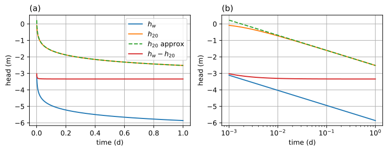
Figure 9.1 Head vs. time for a well in a confined aquifer; \(h_w\) is at the well, and \(h_{20}\) is at \(r = 20\) m; linear time axis (left) and log-scaled time axis (right).

Exercise 9.1

A well starts pumping at time \(t = 0\) in a confined aquifer. After 1 day of pumping, the drawdown is 1 m at a distance of \(r_1 = 20\) m from the well. Compute at what time (in days) after pumping started the drawdown is 1 m at a distance of \(r_2 = 60\) m from the well.

Solution

\(t = 9\) d

Exercise 9.2

Consider a well with discharge \(Q = 300\) m\(^3\)/d that is screened in a confined aquifer with transmissivity \(T = 500\) m\(^2\)/d and storage coefficient \(S = 0.2\). At what distance from the well is the drawdown \(0.2\) m after 1 day of pumping? Hint: use the fsolve function of scipy.optimize.

Solution

\(r = 9.27\) m

Exercise 9.3

Consider a well with discharge \(Q = 300\) m\(^3\)/d and radius \(r_w = 0.3\) m. The well has been pumping in an aquifer with \(T = 500\) m\(^2\)/d and \(S = 0.2\) for 1 day. Compute the water removed from storage by evaluating the integral \(\int_{r_w}^\infty Sh2\pi r\text{d}r\) using a numerical integration function from scipy.integrate. Compare your answer to the total amount of water removed from the aquifer by the well.

Solution

They are the same

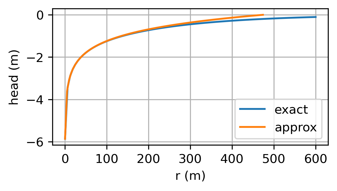
      It may be expected that the head approaches steady state when a well is pumped for a long enough period of time. Strangely enough, this is not the case: The head for a transient well (Eq. (9.9)) does not approach the head for a steady well in an infinite aquifer (Eq. (6.37)) for large time. For a steady well (Eq. (6.37)), the head approaches infinity when \(r\) approaches infinity, because the source of water for a steady well in an infinite aquifer lies at infinity. For a transient well, the head approaches zero when \(r\) approaches infinity. This means that all the water pumped by a transient well in the Theis solution comes from storage. For a single transient well pumping in an infinite aquifer, it is not possible to determine the distance from the well where the drawdown equals zero, because theoretically the drawdown only equals zero at infinity. The drawdown is, obviously, already negligible at a much shorter distance from the well. The distance from the well where the drawdown is negligible can be estimated by rewriting the approximate formula for large time (Eq. (9.14)) in the form of the Thiem equation (Eq. (6.25))

(9.15)\[ h \approx \frac{Q}{2\pi T}\ln(r/R) {\hskip 2em} r\le R \]

where the distance \(R\) is a function of time

(9.16)\[ R = \sqrt{4T(t-t_0)\text{e}^{-\gamma}/S} \]

The distance \(R\) may be used as an approximation of the distance at which the drawdown may be neglected.

Exercise 9.4

Plot the head vs. \(r\) at time \(t = 1\) d for \(r\) varying from \(r_w\) to 600 m using the parameters of the example. On the same graph, plot the approximate formula (9.15).

Solution

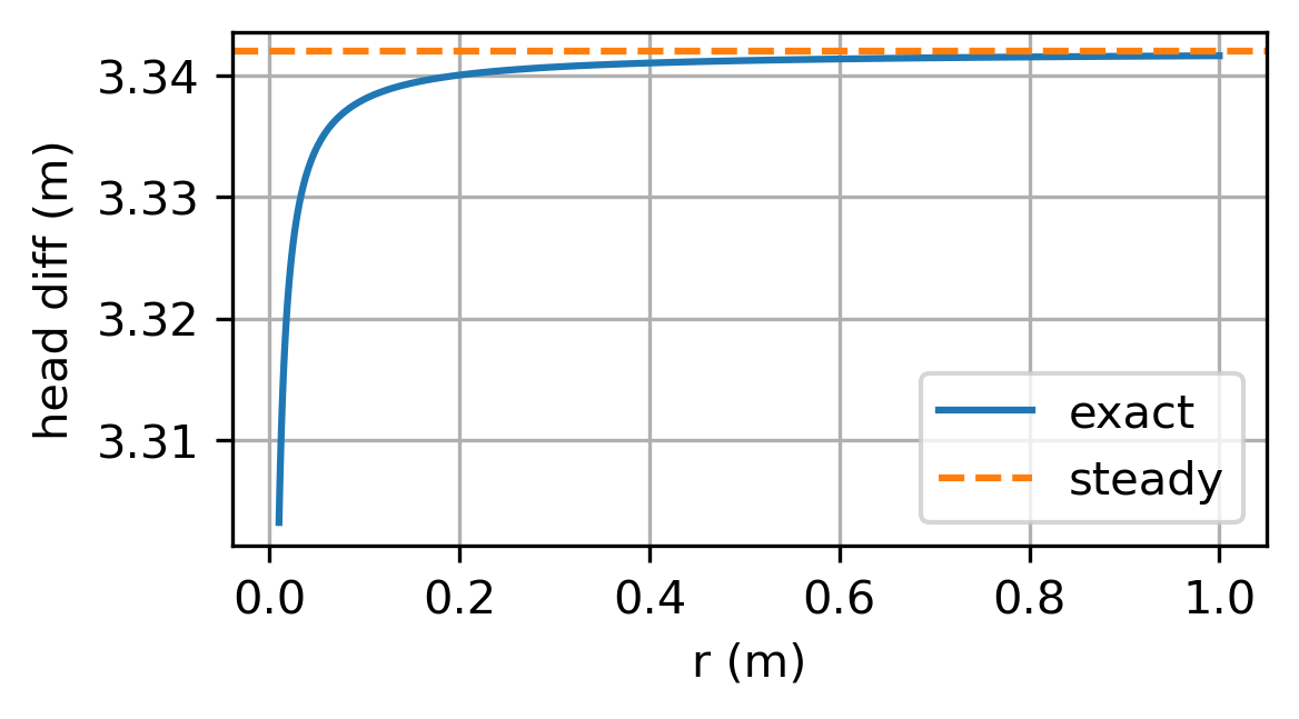
      Even though the head of the Theis solution by itself does not approach the steady-state head of a steady well, the difference between the head at two locations does approach a constant value. This was already shown in Figure 9.1, where the difference in the head between \(r = r_w\) and \(r = 20\) m approaches a constant value for \(t > 0.01\) d (\(u < 0.1\)) for this case. Similarly, the discharge vector approaches the steady solution for small \(u\). The radial component of the discharge vector \(Q_r\) of the Theis solution may be obtained from Eq. ((9.9)) as

(9.17)\[ Q_r = -T\frac{\partial h}{\partial r} = -T\frac{\text{d} h}{\text{d} u}\frac{\partial u}{\partial r} = -\frac{Q}{2\pi} \frac{1}{r}\text{e}^{-u} \]

When time is large, \(u\) approaches zero and \(Q_r\) approaches the steady discharge vector

(9.18)\[ Q_r = -\frac{Q}{2\pi}\frac{1}{r} \]

Exercise 9.5

Compute the steady head difference between \(r = r_w\) and \(r = 20\) m, and compare your answer to the difference obtained with the transient solution for time varying from \(t = 0.01\) to \(t = 1\) d.

Solution

      In practice, there is always a water source closer than infinity, and if that source is included in the solution, the transient solution approaches a steady solution for large time. For example, consider a well at \((x, y) = (−d, 0)\) near a large and straight river with a constant head \(h_0\) along \(x = 0\). The steady solution may be obtained with the method of images (Section 6.2). A transient solution may also be obtained with the method of images as

(9.19)\[ h = -\frac{Q}{4\pi T}\left[ \text{E}_1\left( \frac{S r_1^2}{4T(t-t_0)} \right) - \text{E}_1\left( \frac{S r_2^2}{4T(t-t_0)} \right)\right] + h_0 \]

where \(r_1^2=(x+d)^2+y^2\) and \(r_2^2=(x-d)^2+y^2\). For large time, E\(_1\) may again be represented with the first two terms of the series representation (Eq. (9.13)). Substitution of these terms for E\(_1\) into Eq. ((9.19)) and some algebra leads to the steady solution

(9.20)\[ h=\frac{Q}{2\pi T}\ln\frac{r_1}{r_2} + h_0 \]

Transient solutions may be superimposed in time as well as in space. For example, consider a well with a discharge \(Q\) operating from \(t = t_0\) to \(t = t_1\) and with zero discharge after \(t_1\). For the period \(t > t_1\), the head function consists of two Theis wells, one with discharge \(Q\) starting at \(t = t_0\) and one with discharge \(−Q\) starting at \(t = t_1\)

(9.21)\[ h = -\frac{Q}{4\pi T}\left[ \text{E}_1\left( \frac{S r^2}{4T(t-t_0)} \right) - \text{E}_1\left( \frac{S r^2}{4T(t-t_1)} \right)\right] {\hskip 2em} t \ge t_1 \]

The variation of the head after the well is turned off is called the recovery phase, as the head (slowly) comes back to its original position. For large time, E\(_1\) may again be represented with the first two terms of the series representation of E\(_1\) (Eq. (9.13)), which results in

(9.22)\[ h \approx -\frac{Q}{4\pi T} \ln\left(\frac{t-t_1}{t-t_0}\right) {\hskip 2em} t \gg t_1 \]

This is an important and somewhat surprising result, as the recovery after the well has been turned off for a little while does not depend on the storage coefficient \(S\). In the example below, two solutions are plotted for a well that pumps for one day and is then turned off, but the storage coefficients differ. The head response is quite different during pumping, but the two curves quickly approach each other during the recovery phase, even though the storage coefficients are different. The approximate formula ((9.22)) is also plotted for the recovery phase in Figure 9.2.

# parameters
t0 = 0 # time pump starts, d
t1 = 1 # time pump is turned off, d
S = [1E-3, 1E-4] # storage coefficients, -
r = 100 # m

# solution
t = np.linspace(1e-6, 2, 200)
h = np.zeros((2, len(t)))
for i in range(2):
    h[i] = -Q / (4 * np.pi * T) * exp1(S[i] * r ** 2 / (4 * T * (t - t0)))
    h[i, t > t1] -= -Q / (4 * np.pi * T) * exp1(
        S[i] * r ** 2 / (4 * T * (t[t > t1] - t1)))
tapprox = np.linspace(t1 + 0.01, 2, 100)
happrox = Q / (4 * np.pi * T) * np.log((tapprox - t1) / (tapprox - t0))

# basic plot
plt.plot(t, h[0])
plt.plot(t, h[1])
plt.plot(tapprox, happrox);

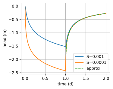
Figure 9.2 Head at \(r = 100\) m for a well that pumps for 1 day and is then turned off; results are shown for two different storage coefficients, and for the approximate solution during the recovery phase (Eq. (9.22)).

      The Theis solution is very useful to estimate aquifer parameters from a pumping test, also called an aquifer test. During a pumping test, a well is turned on and the head (drawdown) is measured in one or more nearby observation wells and/or the pumping well itself. The Theis solution is fitted to the observed heads to estimate the transmissivity \(T\) and the storage coefficient \(S\) of the aquifer.
      Kruseman and De Ridder (1990) described a pumping test at the Oude Korendijk in The Netherlands in their famous book on pumping tests. The objective of the pumping test was to determine the transmissivity and storage coefficient of the aquifer. The discharge of the well during the pumping test was 788 m\(^3\)/day. The observed drawdown (in meters) and the observation time (in minutes) after pumping started are given below for an observation well located 30 m from the pumping well. Kruseman and De Ridder (1990) also reported drawdown in two additional wells, but only one observation well is used here to demonstrate the approach. Time is converted to days, and drawdown is converted to heads.

# Data at Oude Korendijk taken from Kruseman and de Ridder (1990)
robs = 30 # distance to observation well, m
Q = 788 # discharge of well, m^3/d
time = np.array(
    [0.1 ,  0.25,  0.5 ,  0.7 ,  1.  ,  1.4 ,  1.9 ,  2.33,  2.8 ,
     3.36,  4.  ,  5.35,  6.8 ,  8.3 ,  8.7 , 10.  , 13.1 , 18.  ,
     27. ,  33. ,  41. ,  48. ,  59. ,  80. , 95.  , 139. , 181. , 
     245.,  300.,  360.,  480.,  600.,  728., 830.]) # in minutes
drawdown = np.array(
    [0.04 , 0.08 , 0.13 , 0.18 , 0.23 , 0.28 , 0.33 , 0.36 , 0.39 ,
     0.42 , 0.45 , 0.5  , 0.54 , 0.57 , 0.58 , 0.6  , 0.64 , 0.68 ,
     0.742, 0.753, 0.779, 0.793, 0.819, 0.855, 0.873, 0.915, 0.935,
     0.966, 0.99 , 1.007, 1.05 , 1.053, 1.072, 1.088]) # in meters
tobs = time / 24 / 60 # convert observation time to days
hobs = -drawdown # convert drawdown to heads

      First, the measured and modeled heads are plotted on the same graph (Figure 9.3). The left graph has a linear time axis and the right graph a log-scaled time axis. Two sliders are added to adjust the transmissivity and storage coefficient to manually minimize the difference between the measured and modeled values. Next, the values of the transmissivity and the storage coefficient are estimated using a least squares approach by minimizing the sum of squared differences between the modeled heads and the observed heads (similar to the approach in Section 5.3). The objective function fobj returns the sum of squared errors and takes five input arguments: an array of the parameters \(T\) and \(S\), the observed heads, observation times, distance to observation well, and discharge of the well. When the keyword argument return_heads is set to True, the function fobj returns the modeled heads rather than the sum of squared errors.

def fobj(p, ho, to, ro, Q, return_heads=False):
    T, S = p
    hm = htheis(ro, to, T, S, Q)
    if return_heads:
        return hm
    rv = np.sum((ho - hm) ** 2)
    return rv

      The fmin function of the scipy.optimize package is used to find the parameters that minimize the objective function. The four arguments ho, to, ro, and Q of fobj are passed by fmin to the objective function fobj with the args keyword argument of fmin. The fmin function does not estimate the uncertainty of the estimated parameters, but that is not a problem here as standard procedures to estimate the uncertainty are commonly based on certain statistical requirements between the modeled and observed heads that are violated in many pumping test analyses (e.g., the differences between the observed and modeled heads are not independent). Results of the least-squares solution are as follows:

# least squares solution
from scipy.optimize import fmin
T, S = fmin(fobj, [100, 1e-4], args=(hobs, tobs, robs, Q), disp=0)
print(f'Estimated parameters T: {T:.2f} m^2/d, S: {S:.2e}')
hm = fobj([T, S], hobs, tobs, robs, Q, return_heads=1) # compute modeled heads
rmse = np.sqrt(np.mean((hobs - hm) ** 2))
print(f'Root mean squared error: {rmse:.3f} m')

Estimated parameters T: 480.47 m^2/d, S: 1.13e-04
Root mean squared error: 0.032 m

# basic plot
plt.subplot(121)
plt.plot(tobs, hobs, 'C1.')
plt.plot(tobs, hm, 'C0')
plt.subplot(122)
plt.semilogx(tobs, hobs, 'C1.')
plt.semilogx(tobs, hm, 'C0');

Figure 9.3 A pumping test analysis; linear time axis (left) and log-scaled time axis (right).

Exercise 9.6

Consider a pumping test for a well that is located 30 m from a river. Measurements are taken in an observation well located 5 m from the well and 25 m from the river. Hourly measurements of a 20-hour pumping test are given below. The discharge of the well was 200 m\(^3\)/d. Estimate the transmissivity and storage coefficient of the aquifer from the pumping test first by neglecting the presence of the river and second by including the river using the method of images.

Solution

\(T = 256\) m\(^2\)/d, \(S = 0.057\) without river
\(T = 197\) m\(^2\)/d, \(S = 0.107\) with river

tobs = np.array([1, 2, 3, 4, 5, 6, 7, 8, 9, 10,    # time in hours
    11, 12, 13, 14, 15, 16, 17, 18, 19, 20]) 
hobs = np.array(                                   # head change in m
    [-0.16, -0.22, -0.24, -0.27, -0.28, -0.29, -0.31, -0.31, -0.32, -0.32, 
     -0.33, -0.33, -0.34, -0.34, -0.35, -0.35, -0.34, -0.34, -0.35, -0.35])