5.2. Periodic changes in surface water level

Periodic head variations in an aquifer may be caused by, e.g., tides, seasonal fluctuations, or the periodic operation of dams. The surface water level variation is approximated here as a sinusoidal fluctuation with one specific amplitude and one specific period. Surface water level variations can commonly be expressed as a combination of several sinusoidal fluctuations with their own amplitude and period; the response to such a combined variation may be computed through superposition.
     Consider one-dimensional flow in a semi-infinite aquifer (see Figure 5.6). There is no areal recharge and no flow at infinity

(5.32)\[ \left. \frac{\partial h}{\partial x}\right\vert_{x\to\infty, t} = 0 \]

The transmissivity \(T\) of the aquifer is approximated as constant. The aquifer is bounded by open water at \(x=0\), which fluctuates as

(5.33)\[ h\vert_{x=0, t} = A\cos\left( \frac{2\pi(t-t_p)}{\tau}\right) \]

where \(A\) is the amplitude of the fluctuation, \(t_p\) is the time of the peak, and \(\tau\) is the period of the fluctuation. There is no initial condition; that is, the head at \(x=0\) has fluctuated as ((5.33)) forever (in practice, for a long time).

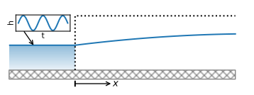
Figure 5.6 Groundwater response to periodic changes in surface water level.

     The solution to the stated problem may be obtained with separation of variables and was first published by Forchheimer (1919, p. 1229). It turns out that the head response in the aquifer may be written in the same form as the head variation in the surface water, but the amplitude \(B\) of the variation is smaller than \(A\) and the peak arrives \(t_s\) later (Jacob, 1950, p. 365)

(5.34)\[ h(x, t) = B(x) \cos[2\pi(t-t_p-t_s)/\tau] \]

The amplitude \(B\) of the head variation dampens with distance as

(5.35)\[ B = A\exp\left(-x\sqrt{\frac{S\pi}{T\tau}}\right) \]

and the time shift \(t_s\) of the peak is

(5.36)\[ t_s = x\sqrt{\frac{S\tau}{4\pi T}} \]

Note that both the amplitude \(B\) and the phase shift \(t_s\) are a function of the diffusivity \(T/S\). This means that when the amplitude and peak time of a tidal response are measured to estimate aquifer parameters, only the aquifer diffusivity can be estimated, not the individual values of \(S\) or \(T\). Estimation of (combinations of) aquifer parameters from the tidal response is also referred to as the tidal method (e.g., Ferris, 1952; Carr and Van Der Kamp, 1969).
     Equation ((5.35)) shows that the amplitude \(B\) dampens out more quickly for shorter tidal periods than for longer tidal periods. The characteristic length \(\mu\) is introduced as

(5.37)\[ \mu = \sqrt{\frac{T\tau}{S\pi}} \]

so that the amplitude may be written as

(5.38)\[ B = A\text{e}^{-x/\mu} \]

At a distance of \(x=3\mu\), the amplitude has dampened to 5% of the amplitude at \(x=0\). This result may be used as a rule of thumb to assess whether periodic fluctuations in surface water levels need to be taken into account when considering the head and flow in an aquifer. If the area of interest is farther away from a surface water body than \(3\mu\), periodic fluctuations of the surface water level with a period of \(\tau\) may be neglected.
     As an example, consider an aquifer bounded by a tidal river. The head in the aquifer is plotted at four different times during one tidal period (Figure 5.7). The amplitude in the river is set to 1 m. The head variation is bounded by the amplitude \(B\), which is shown with the dashed line in the code below. The solution is shown with an animation.

# parameters
T = 1000 # transmissivity, m^2/d
S = 0.1 # storate coefficient, -
tau = 0.5 # tidal period, d
tp = 0 # time of peak at canal, d
mu = np.sqrt(T * tau / (S * np.pi)) # characteristic length, m
print(f'characteristic length: {mu:.2f} m')

characteristic length: 39.89 m

# solution for unit amplitude
def head(x, t, tau, S, T, tp=0, t0=0):
    B = np.exp(-x * np.sqrt(S * np.pi / (T * tau)))
    ts = x * np.sqrt(S * tau / (4 * np.pi * T))
    return B * np.cos(2 * np.pi * (t - tp - ts) / tau)

# basic plot
x = np.linspace(0, 200, 100)
for t in np.arange(0, tau, tau / 4):
    h = head(x, t, tau, S, T, tp)
    plt.plot(x, h)
plt.plot(x, np.exp(-x / mu), 'k--')
plt.plot(x, -np.exp(-x / mu), 'k--');

Once Loop Reflect

Figure 5.7 Tidal response in an aquifer.

     Natural tidal fluctuations consist of a number of tidal components, each with its own period and phase lag. As an example, the response is presented to a tidal fluctuation consisting of two components. The first component is a semidiurnal component with a period of 745 minutes (referred to as component M2 in the system of tides); the amplitude of M2 is 1 m. The second component is a diurnal component with a period of 1549 minutes (referred to as component O1). The amplitude of O1 is 0.4 m, and the phase lag compared to M2 is 100 minutes. The solution is obtained through superposition of two solutions ((5.34)). The head fluctuation is computed at the shoreline and in three observation wells at three different distances from the coast line (Figure 5.8).
     The presence of just two components causes the head fluctuation to become already quite complicated. The head fluctuates more than 2 m at the coast, while the variation at \(x=300\) m is only 5 mm. Component M2 damps out quicker than O2 as the period of M2 is smaller than the period of O2. The tidal fluctuation has two clear peaks near the coast, while there is only one clear peak farther away from the coast.

# parameters
tau1 = 745 / (24 * 60) # M2 period, d
tau2 = 1549 / (24 * 60) # O1 period, d
tp1 = 0 # time of peak M2, d
tp2 = 100 / (24 * 60) # time of peak of O1, d
mu1 = np.sqrt(T * tau1 / (S * np.pi)) # characteristic length M2, m
mu2 = np.sqrt(T * tau2 / (S * np.pi)) # characteristic length O1, m
print(f'characteristic length M2: {mu1:.2f} m')
print(f'characteristic length O1: {mu2:.2f} m')

characteristic length M2: 40.58 m
characteristic length O1: 58.52 m

# basic plot
t = np.linspace(0, 4, 400)
for i, x in enumerate([0, 100, 200, 300]):
    h = 1 * head(x, t, tau1, S, T, tp1) + \
        0.4 * head(x, t, tau2, S, T, tp2)
    plt.subplot(2, 2, i + 1)
    plt.plot(t, h)

Once Loop Reflect

Figure 5.8 Tidal response to a tide consisting of two components. Fluctuation of the surface water (blue) and in two observation wells (orange and green).