6. Steady two-dimensional flow to wells

Many three-dimensional groundwater flow problems can be approximated as two-dimensional in the horizontal plane through adoption of the Dupuit–Forchheimer approximation. Of particular interest are problems that include wells. In this chapter, solutions are presented for extraction wells, injection wells, and wells near rivers and impermeable boundaries. Different solution techniques are demonstrated, depending on the type of problem. For homogeneous confined and unconfined aquifers, solutions are formulated in terms of a discharge potential so that the same potential solution can be used for confined flow, unconfined flow, and interface flow. The stream function is used in the horizontal plane for problems without areal infiltration. Solutions for flow to wells in semi-confined aquifers and two-aquifer systems are formulated in terms of heads.

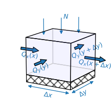
Figure 6.1 Two-dimensional water balance.

      The discharge vector for two-dimensional flow in the horizontal plane consists of two components: \(Q_x\) in the \(x\)-direction and \(Q_y\) in the \(y\)-direction (Figure 6.1). Continuity of flow for steady two-dimensional flow in the horizontal \(x, y\) plane may be written as

(6.1)\[ \frac{\partial Q_x}{\partial x} + \frac{\partial Q_y}{\partial y} = N \]

where \(N\) is the areal recharge. Note that this equation differs from the continuity of flow equation for one-dimensional steady flow (Eq. (1.5)) only by the additional term \(\partial Q_y / \partial y\).
      Steady confined, unconfined, and interface flows may be formulated as potential flow, where the discharge vector is minus the gradient of the discharge potential

(6.2)\[ Q_x = -\frac{\partial \Phi}{\partial x} \quad\quad Q_y = -\frac{\partial \Phi}{\partial y} \]

so that the differential equation for steady potential flow becomes the two-dimensional Poisson equation

(6.3)\[ \nabla^2 \Phi = \frac{\partial^2 \Phi}{\partial x^2} + \frac{\partial^2 \Phi}{\partial y^2} = -N \]

In the absence of areal recharge (\(N = 0\)), this differential equation is referred to as the two-dimensional Laplace equation. The relationships between the discharge potential and head for different flow types are summarized in Table 6.1.

Table 6.1 Definition of the discharge potential for different types of flow where \(k\) is the hydraulic conductivity of the aquifer, \(z_b\) and \(z_t\) are the elevations of the bottom and top of the aquifer, \(H\) is the aquifer thickness, and \(\alpha=\rho_f/(\rho_s - \rho_f)\), where \(\rho_f\) and \(\rho_s\) are the densities of freshwater and saltwater, respectively. For interface flow, all heads and elevations are measured with respect to sea level.

Flow Type	Discharge potential	Condition	Section
Confined flow	\(\Phi = kHh\)	\(h \ge z_t\)	3.3
Unconfined flow	\(\Phi = \tfrac{1}{2}k(h-z_b)^2\)	\(h \ge z_b\)	3.1
Confined/unconfined flow	\(\Phi = kHh -(\tfrac{1}{2}kH^2 + kHz_b)\)	\(h \ge z_t\)	3.3
	\(\Phi = \tfrac{1}{2}k(h-z_b)^2\)	\(z_b \le h \le z_t\)	3.3
Confined interface flow	\(\Phi = kHh + (\tfrac{1}{2} kH^2 + kHz_b) / \alpha\)	\(h\ge -z_b/\alpha\)	4.1
	\(\Phi = \tfrac{1}{2}k\alpha(h+z_t/\alpha)^2\)	\(-z_t/\alpha\le h\le -z_b/\alpha\)	4.1
Unconfined interface flow	\(\Phi = \tfrac{1}{2}k(h-z_b)^2 -\tfrac{1}{2}k(\alpha+1)z_b^2 / \alpha\)	\(h\ge -z_b/\alpha\)	4.2
	\(\Phi = \tfrac{1}{2}k(\alpha+1)h^2\)	\(0\le h \le -z_b/\alpha\)	4.2

      Flow to a pumping well in a homogeneous, isotropic aquifer is radially symmetric in the absence of any other flow features. As a result, the head and flow are a function only of the radial distance to the well. The continuity equation in terms of radial coordinates is derived by considering the water balance for an annulus (Figure 6.2). The inner radius of the annulus is \(r\), the outer radius is \(r + \Delta r\), and \(Q_r\) is the radial component of the discharge vector (i.e., positive away from the well). For steady flow, the continuity equation is

(6.4)\[ \text{Inflow} - \text{Outflow} = 0 \]

Inflow equals areal recharge on the annulus and inflow along the inner radius. Outflow equals outflow along the outer radius so that the continuity equation becomes

(6.5)\[ (\pi(r + \Delta r)^2 - \pi r^2)N + 2\pi rQ_r|_r - 2\pi(r + \Delta r)Q_r|_{r + \Delta r} = 0 \]

Division by \(2\pi \Delta r\) and taking the limit for \(\Delta r \to 0\) gives

(6.6)\[ Nr -\frac{\text{d}(rQ_r)}{\text{d}r} = 0 \]

Application of the product rule for differentiation and using that the radial component of the discharge vector is

(6.7)\[ Q_r = -\frac{\text{d}\Phi}{\text{d} r} \]

gives the differential equation for steady potential flow in radial coordinates

(6.8)\[ \frac{\text{d}^2\Phi}{\text{d} r^2}+\frac{1}{r}\frac{\text{d}\Phi}{\text{d}r} = -N \]

Note that this equation is consistent with Eq. ((6.3)) because the Laplacian in terms of polar coordinates \(r,\theta\) is

(6.9)\[ \nabla^2 \Phi = \frac{\partial^2\Phi}{\partial r^2}+\frac{1}{r}\frac{\partial\Phi}{\partial r} + \frac{1}{r^2} \frac{\partial^2\Phi}{\partial \theta^2} \]

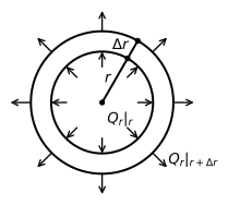
Figure 6.2 Continuity of flow for radially symmetric flow.

In radial coordinates there is no dependence on \(\theta\) so that the derivative with respect to \(\theta\) drops out and the partial derivatives become ordinary derivatives.
      In Chapters 1–4, the stream function was computed in the vertical plane for one-dimensional Dupuit–Forchheimer flow. Recharge entered the vertical plane through the boundaries, and flow in the vertical plane was divergence-free (Eq. (1.28)). The lower case symbol \(\psi\) [L\(^2\)/T] was used for the stream function in the vertical plane.
      The stream function also exists for steady two-dimensional Dupuit-Forchheimer flow in the horizontal plane if the flow is divergence-free. In the horizontal plane, flow is divergence-free if the areal recharge \(N\) equals zero

(6.10)\[ \frac{\partial Q_x}{\partial x} + \frac{\partial Q_y}{\partial y} = 0 \]

so that the discharge potential is governed by Laplace’s equation

(6.11)\[ \nabla^2 \Phi = 0 \]

In the horizontal plane, the upper case symbol \(\Psi\) is used for the stream function, which has dimensions L\(^3\)/T.
      For two-dimensional flow in the horizontal plane, the components of the discharge vector can be obtained from the stream function, as is explained in the following. Recall that the stream function is defined by three characteristics: The stream function is a function that is constant along streamlines, the difference of the stream function values between two points is equal to the amount of water flowing between the two points, and the value of the stream function increases to the right when looking in the direction of flow. Consider points \(A\), \(B\), and \(C\) shown in Figure 6.3. Water flows from left to right across \(AB\). The component of the discharge vector normal to \(AB\) is \(Q_x\), the distance between \(A\) and \(B\) is \(\Delta y\), and the difference in the stream function between \(A\) and \(B\) is \(\Delta \Psi\) so that

(6.12)\[ Q_x \Delta y = \Delta \Psi = \Psi(x,y) - \Psi(x, y + \Delta y) \]

hence

(6.13)\[ Q_x = -\frac{\Psi(x,y + \Delta y) - \Psi(x, y)}{\Delta y} \]

In the limit for \(\Delta y\) to zero, this gives

(6.14)\[ Q_x= -\frac{\partial \Psi}{\partial y} \]

Similarly, water flows from bottom to top across \(BC\). The component of the discharge vector normal to \(BC\) is \(Q_y\), the distance between \(B\) and \(C\) is \(\Delta x\), and the difference in the stream function between \(B\) and \(C\) is \(\Delta \Psi\), so that

(6.15)\[ Q_y \Delta x = \Delta \Psi = \Psi(x + \Delta x,y) - \Psi(x, y) \]

and hence

(6.16)\[ Q_y = \frac{\partial \Psi}{\partial x} \]

Comparison of Eqs. ((6.14)) and ((6.16)) with Eq. ((6.2)) gives

(6.17)\[ \begin{align}\begin{aligned} &\frac{\partial \Phi}{\partial x} = \frac{\partial \Psi}{\partial y}\\&\frac{\partial \Phi}{\partial y} = -\frac{\partial \Psi}{\partial x} \end{aligned}\end{align} \]

This set of two equations is known as the Cauchy–Riemann conditions. Since the discharge potential and stream function fulfill the Cauchy–Riemann conditions, they can be combined into a complex potential, as is explained in Section 7.5.

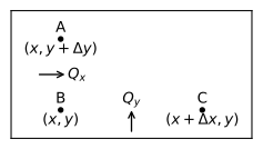
Figure 6.3 Flow between points A-B and B-C used in the derivation of the stream function.

      The discharge potential is a single-valued function, which means that the discharge potential has only one value at a point. A mathematical definition of a single-valued function is (e.g., Strack, 1989)

(6.18)\[ \frac{\partial^2 \Phi}{\partial x \partial y} = \frac{\partial^2 \Phi}{\partial y \partial x} \]

Application of the Cauchy-Riemann conditions ((6.17)) to replace \(\Phi\) by \(\Psi\) in Eq. ((6.18)) gives

(6.19)\[ \frac{\partial^2 \Psi}{\partial x^2} + \frac{\partial^2 \Psi}{\partial y^2} = 0 \]

This is a nice result, because it means that the stream function is governed by Laplace’s equation, just like the discharge potential (Eq. (6.11)). Recall that the stream function in the horizontal plane only exists when the areal recharge \(N\) equals zero.