2.1. Flow from a canal to a drained area

Consider one-dimensional flow from a canal into a polder. The aquifer is semi-confined and semi-infinite, and is bounded on the left by a fully penetrating canal with water level \(h_l\), as shown in Figure 2.2; the head in the polder is fixed to \(h^*\). The governing differential equation is the modified-Helmholtz equation, as derived above. The boundary conditions are

(2.11)\[\begin{split} \begin{split} &h\vert_{x=0}=h_l \\ &h\vert_{x\to\infty}=h^* \end{split} \end{split}\]

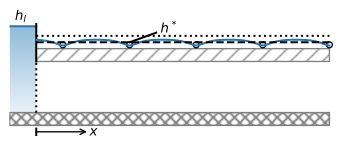
Figure 2.2 Semi-confined flow from a canal to a polder.

Application of the second boundary condition gives \(B=0\), after which application of the first boundary condition gives \(A=h_l-h^*\), so that the solution for \(h\) becomes

(2.12)\[ h = h^* + (h_l-h^*)\text{e}^{-x/\lambda} \]

Water flows from the canal into the semi-confined aquifer and then through the leaky layer into the overlying polder (provided that the head in the canal is larger than the head in the polder). The discharge vector in the aquifer is

(2.13)\[ Q_x = -T\frac{\text{d}h}{\text{d}x}=\frac{T(h_l-h^*)}{\lambda}\text{e}^{-x/\lambda} \]

An example solution is shown below (Figure 2.3). Equations ((2.12)) and ((2.13)) for \(h\) and \(Q_x\) are implemented in Python functions so that they can easily be re-used later on in this section.

# parameters
hstar = 0 # head above leaky layer, m
hl = 1 # specified head at the left boundary, m
k = 10 # hydraulic conductivity, m/d
H = 40 # aquifer thickness, m
c = 100 # resistance of leaky layer, d
T = k * H # transmissivity, m^2/d
lab = np.sqrt(c * T) # leakage factor, m
print(f'the leakage factor is: {lab:.0f} m')

the leakage factor is: 200 m

# solution
def head(x):
    return (hl - hstar) * np.exp(-x / lab) + hstar

def disvec(x):
    return k * H * (hl - hstar) / lab * np.exp(-x / lab)

x = np.linspace(0, 5 * lab, 100)
h = head(x)
Qx = disvec(x)

# basic plot
plt.subplot(121)
plt.plot(x, h, 'C0')
plt.subplot(122)
plt.plot(x, Qx, 'C1');

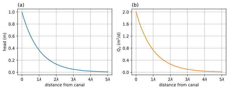
Figure 2.3 Semi-confined flow from a canal to a polder; \(\lambda\) is the leakage factor; head (left) and \(Q_x\) (right).

      The total discharge per meter length of canal normal to the plane of flow is called \(Q_l\) and is obtained by evaluating \(Q_x\) at \(x=0\), which gives \(Q_l=T(h_l-h^*)/\lambda\). The discharge vector \(Q_x\) in the aquifer decreases with distance from the canal, as groundwater discharges across the leaky layer into the drainage system of the polder. At a distance \(x=\lambda\), \(Q_x\) has reduced to \(\text{e}^{-1}Q_l=0.37Q_l\), and at a distance \(x=3\lambda\), \(Q_x\) has reduced to only \(\text{e}^{-3}Q_l=0.05Q_l\). Hence, 95% of the water that flows from the canal into the aquifer has discharged into the polder within a distance of \(3\lambda\) from the canal. That is why the leakage factor \(\lambda\) is also called a characteristic length of the system. Similarly, the difference between the head in the aquifer and the head in the polder reduces from \(h_l-h^*\) at the canal (\(x=0\)) to only \(0.05(h_l-h^*)\) at \(x=3\lambda\). Roughly speaking, three times the leakage factor away from the canal, the head in the aquifer is approximately equal to the head \(h^*\) above the semi-confined aquifer.
      Several checks may be conducted to verify that the solution and its Python implementation (the functions head and disvec) are correct. First, it is verified that the solution meets the boundary conditions in Eq. ((2.11)).

# Verify boundary conditions
print(f'head at x=0: {head(0):.0f} m')
print(f'head at x=infinity: {head(np.inf):.0f} m')

head at x=0: 1 m
head at x=infinity: 0 m

      Second, it is verified that the solution meets the governing differential equation (2.5) using an accurate numerical approximation of the second derivative

(2.14)\[ \frac{\text{d}^2h}{\text{d}x^2} \approx \frac{h|_{x - \Delta x} - 2h|_x + h|_{x + \Delta x}}{(\Delta x)^2} \]

where \(\Delta x\) is a suitably small increment.

# Verify differential equation
x = 200 # example point where deq is checked
delx = 0.001
left_side = (head(x - delx) - 2 * head(x) + head(x + delx)) / delx ** 2
right_side = (head(x) - hstar) / lab ** 2
print(f'left_side of deq : {left_side}')
print(f'right_side of deq: {right_side}')

left_side of deq : 9.196976513692334e-06
right_side of deq: 9.196986029286058e-06

      Third and final, it is checked that the specific discharge is indeed \(Q_x=-T\text{d}h/\text{d}x\) using the numerical derivative

(2.15)\[ \frac{\text{d}h}{\text{d}x} \approx \frac{h|_{x + \Delta x} - h|_{x - \Delta x}}{2\Delta x} \]

# Verify Qx
Qx = disvec(x)
Qxnum = -T * (head(x + delx) - head(x - delx)) / (2 * delx)
print(f'Qx exact               : {Qx} m^2/d')
print(f'Qx numerical derivative: {Qxnum} m^2/d')

Qx exact               : 0.7357588823428847 m^2/d
Qx numerical derivative: 0.7357588823531103 m^2/d

      It is important to perform the above three checks to verify a solution. If the solution is correct (and correctly programmed), the solution and the approximation using numerical derivatives must be approximately equal.The number of significant digits that match depends on the size of the increment \(\Delta x\) and on machine accuracy.

Exercise 2.1

Consider the case of the example, but this time the resistance \(c\) is unknown. The head in the aquifer is measured in an observation well at \(x=100\) m, where the head is 0.5 m. Compute the resistance and the leakage factor.

Solution

\(\lambda = 144.3\) m
\(c=52.0\) d

Exercise 2.2

Verify that the total flux from the canal into the aquifer \((Q_l)\) is equal to the integrated leakage through the leaky layer by analytic integration of \(q_z\).

Solution

\(\left.Q_x\right|_{x=0}=T(h_l - h^*) / \lambda=\int_0^\infty q_zdx\)