3.2. Flow over a step in the aquifer base

The problem of unconfined flow between two parallel rivers without areal recharge is considered, but this time, there is a step in the base of the aquifer as shown in Figure 3.6. The base of the aquifer is equal to \(z_0\) for the left part of the aquifer (length \(L_0\)) and is equal to \(z_1\) for the right part of the aquifer (length \(L_1\)). The head is \(h_l\) at \(x =0\), and the head is \(h_r\) at \(x=L\). These conditions are transformed to conditions in terms of the discharge potential

(3.20)\[ \Phi\vert_{x=0}=\Phi_l=\tfrac{1}{2}k(h_l-z_0)^2 \]

(3.21)\[ \Phi\vert_{x=L}=\Phi_r=\tfrac{1}{2}k(h_r-z_1)^2 \]

As for the solution of, e.g., Section 1.4, the head and flux are continuous at \(x=L_0\)

(3.22)\[ h^-=h^+ \]

(3.23)\[ Q_x^-=Q_x^+ \]

where the superscripts \(^-\) and \(^+\) are used as shorthand for evaluation just to the left and right of \(x=L_0\), respectively.

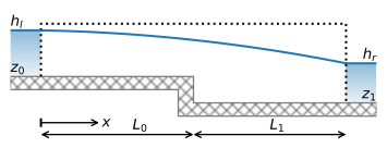
Figure 3.6 Unconfined flow with a step in the base.

     The flow from the left river to the right river is equal to \(U\), which is unknown upfront. Application of boundary conditions ((3.20)) and ((3.21)) gives equations for the discharge potential for the left and right parts that still contain the unknown flux \(U\)

(3.24)\[ \Phi=-Ux + \Phi_l \hskip 2em 0 \le x \le L_0 \]

(3.25)\[ \Phi=-U(x-L) + \Phi_r \hskip 2em L_0 \le x \le L \]

where \(L=L_0+L_1\). The discharge \(U\) is obtained from condition ((3.22)) as follows. The discharge potentials \(\Phi^-\) and \(\Phi^+\) at \(x=L_0\) are

(3.26)\[ \Phi^- = -UL_0 + \Phi_l = \tfrac{1}{2}k(h^- -z_0)^2 \]

(3.27)\[ \Phi^+ = -U(L_0 - L) + \Phi_r = \tfrac{1}{2}k(h^+ -z_1)^2 \]

which are transformed in the following expressions for \(h^-\) and \(h^+\)

(3.28)\[ h^- = \sqrt{\frac{2(-UL_0+\Phi_l)}{k}} + z_0 \]

(3.29)\[ h^+ = \sqrt{\frac{2(UL_1+\Phi_r)}{k}} + z_1 \]

Setting \(h^-=h^+\) gives an equation from which \(U\) can be determined, but it is not possible to write an explicit equation for \(U\). The value of \(U\) for which \(h^-=h^+\) is determined numerically. First, \(h^-\) and \(h^+\) are plotted vs. \(U\) in Figure 3.7.

# parameters
k = 10 # hydraulic conductivity, m/d
z0 = 0 # base elevation left section, m
z1 = -4 # base elevation right section, m
L0 = 500 # length of left section, m
L1 = 500 # length of right section, m
L = L0 + L1 # total distance between rivers, m
hl = 10 # specified head at the left boundary, m
hr = 0 # specified head at the right boundary, m

# solution
phil = 0.5 * k * (hl - z0)**2
phir = 0.5 * k * (hr - z1)**2

def hmin(U, L0=L0, z0=z0, phil=phil):
    return np.sqrt(2 * (-U * L0 + phil) / k) + z0

def hplus(U, L1=L1, z1=z1, phir=phir):
    return np.sqrt(2 * (U * L1 + phir) / k) + z1

# basic plot two conditions
U = np.linspace(0, 1, 100)
plt.plot(U, hmin(U), label='$h^-$')
plt.plot(U, hplus(U), label='$h^+$')
plt.legend();

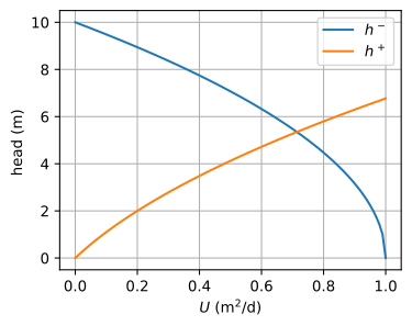
Figure 3.7 Head at \(x=L_0\) vs. \(U\).

     As can be seen from the graph in Figure 3.7, the lines for \(h^-\) and \(h^+\) intersect somewhere between \(U=0.6\) m\(^2\)/d and \(U=0.8\) m\(^2\)/d. To determine the intersection point, a Python function is written to compute the difference between \(h^-\) and \(h^+\) for a given value of \(U\). The value of \(U\) for which this function is zero (so that \(h^-=h^+\)) is found with the fsolve method of the scipy.optimize package

from scipy.optimize import fsolve

def hdiff(U):
    return hmin(U) - hplus(U)

U = fsolve(hdiff, 0.7)[0]  # first value of array returned by fsolve
print(f'U: {U:0.4f} m^2/d')

U: 0.7139 m^2/d

     The head can be computed with Eqs. ((3.28)) and ((3.29)) now that \(U\) is known. The water table and streamlines in a vertical cross section are plotted in Figure 3.8. Note that the water table is continuous, but its slope (i.e., the head gradient) is not. This makes sense as the saturated thickness suddenly increases at the change in base while the discharge vector is continuous. This is only possible if at the same point the head gradient suddenly decreases. The elevations of the streamlines in Figure 3.8 jump at the change in the base. Both the jump in head gradient and the jumps in the streamlines are a consequence of the Dupuit–Forchheimer approximation, which means that streamlines can shift up or down without the loss of energy. In reality, the transition of both the head and the streamlines across a step in the base is smooth, as is demonstrated in Section 10.3.

# solution
x = np.hstack((np.linspace(0, L0 - 1e-6, 100), np.linspace(L0 + 1e-6, L, 100)))
phi = np.empty_like(x)
phi[x < L0] = -U * x[x < L0] + phil
phi[x >= L0] = -U * (x[x >= L0] - L) + phir
h = np.zeros_like(phi)
h[x < L0] = np.sqrt(2 * phi[x < L0] / k) + z0
h[x >= L0] = np.sqrt(2 * phi[x >= L0] / k) + z1
#
psi = np.zeros((2, len(x)))
psi[1] = -U
xg = np.zeros_like(psi)
xg[:] = x
zg = np.zeros_like(xg)
zg[0, :100] = z0
zg[0, 100:] = z1
zg[1] = h

# basic streamline plot
plt.subplot(111, aspect=25)
plt.contour(xg, zg, psi, np.linspace(-U, 0, 4), colors='C1', linestyles='-')
plt.plot(x, h, 'C0')
plt.plot(x, zg[0], 'k');

Figure 3.8 Streamlines for unconfined flow over a step in the base. Discharge between two streamlines is \(\Delta\psi=U/3\).