8.2. Line-sinks for modeling rivers and streams

Pumping wells are sometimes referred to as point-sinks because they take water out at a point (fully penetrating wells take water out over the entire aquifer thickness, which is a point in the two-dimensional horizontal plane). Line-sinks take out water along a line segment and may be used to simulate groundwater flow to or from sections of narrow rivers, streams, or canals. The analytic element code developed in the previous section is extended to include line-sinks. All analytic element classes Model, Element, HeadEquation, Constant, UniformFlow, Well, and HeadWell, defined in section Section 8.1 , are required to run the examples in this section.

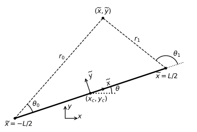
Figure 8.4 The local coordinate system for a line-sink.

     The potential for a line-sink with uniform inflow may be obtained by integrating the potential for a point-sink (a well) along a line. A local \(\tilde{x},\tilde{y}\) coordinate system is introduced (see Figure 8.4). The origin of the local coordinate system is at the center of the line-sink and the \(\tilde{x}\) axis is along the line-sink. Coordinates in the local coordinate system may be computed as

(8.8)\[\begin{split} \begin{split} \tilde{x} &= (x-x_c)\cos(\theta) + (y-y_c)\sin(\theta) \\ \tilde{y} &= -(x-x_c)\sin(\theta) + (y-y_c)\cos(\theta) \end{split} \end{split}\]

where \(x_c,y_c\) is the center of the line-sink and \(\theta\) is the angle between the line-sink and the positive \(x\)-axis (see Figure 8.4). The potential for a line-sink is

(8.9)\[ \Phi = \frac{\sigma}{2\pi} [(\tilde{x}+\tfrac{L}{2})\ln(r_0) - (\tilde{x}-\tfrac{L}{2})\ln(r_1) -\tilde{y}\theta_0 +\tilde{y}\theta_1] \]

where \(\sigma\) is the inflow into the line-sink (the discharge per unit length of line-sink, positive for taking water out of the aquifer), \(L\) is the length of the line-sink, \(r_0\) and \(r_1\) are the distances between \(\tilde{x},\tilde{y}\) and the endpoints of the line-sink, and \(\theta_0\) and \(\theta_1\) are the angles with respect to the endpoints of the line-sink, as shown in Figure 8.4. The total discharge \(Q\) of the line-sink is \(Q=\sigma L\).
     Line-sinks are added to the analytic element code for wells and uniform flow developed previously. Input arguments are the model to which the element is added, the coordinates of the endpoints, and the inflow \(\sigma\). The LineSink class has one function: the potinf function, which implements Eq. ((8.9)) for \(\sigma=1\). The potential ((8.9)) for a line-sink cannot easily be computed at the end points, because either \(r_0\) or \(r_1\) equals zero, but the discharge potential is finite because when \(r_0=0\) then also \(x=-L/2\) and when \(r_1=0\) then \(x=L/2\). The value of \((Z-1)\) or \((Z+1)\) is set to \(10^{-12}\) when their absolute value is smaller than \(10^{-12}\) using the np.where function in the code below.

class LineSink(Element):
    
    def __init__(self, model, x0=0, y0=0, x1=1, y1=1, sigma=1):
        Element.__init__(self, model, sigma)
        self.x0, self.y0 = x0, y0
        self.x1, self.y1 = x1, y1
        self.xc = 0.5 * (self.x0 + self.x1)
        self.yc = 0.5 * (self.y0 + self.y1)
        self.L = np.sqrt((self.x1 - self.x0) ** 2 + (self.y1 - self.y0) ** 2)
        self.theta = np.arctan2(self.y1 - self.y0, self.x1 - self.x0)
    
    def potinf(self, x, y):
        xt = (x - self.xc) * np.cos(self.theta) + (y - self.yc) * np.sin(self.theta)
        yt = -(x - self.xc) * np.sin(self.theta) + (y - self.yc) * np.cos(self.theta)
        r0 = np.sqrt((xt + self.L / 2) ** 2 + yt ** 2)
        r1 = np.sqrt((xt - self.L / 2) ** 2 + yt ** 2)
        r0 = np.where(r0 < 1e-12, 1e-12, r0)
        r1 = np.where(r1 < 1e-12, 1e-12, r1)
        theta0 = np.arctan2(yt, xt + self.L / 2)
        theta1 = np.arctan2(yt, xt - self.L / 2)
        pot = 1 / (2 * np.pi) * (
            (xt + self.L / 2) * np.log(r0) - (xt - self.L / 2) * np.log(r1) - yt * theta0 + yt * theta1)
        return pot

As a first example, the equipotentials of a single line-sink are plotted in the left graph of Figure 8.5. The branch cut starts at the first point of the line-sink and extends to infinity in the same direction as the line-sink. The variation of the head along the line-sink is plotted in the right graph of Figure 8.5.

# parameters and model
ml = Model(T=100) # transmissivity, m^2/d
ls1 = LineSink(ml, x0=-200, y0=-150, x1=200, y1=150, sigma=0.1) # sigma, m^2/d

# solution
xg, yg = np.meshgrid(np.linspace(-400, 400, 100), np.linspace(-300, 300, 100))
h = ml.head(xg, yg)
xs, ys = np.linspace(-200, 200, 100), np.linspace(-150, 150, 100)
hs = ml.head(xs, ys) # head along line-sink

# basic plot
plt.subplot(121, aspect=1)
plt.contour(xg, yg, h, 10)
plt.plot([-200, 200], [-150, 150], 'k')
plt.subplot(122)
plt.plot(np.sqrt((xs + 200) **2 + (ys + 150) ** 2), hs);

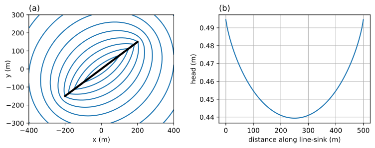
Figure 8.5 Equipotentials of single line-sink with uniform inflow (left) and head along line-sink (right).

The inflow is uniform along a line-sink, which results in a head that varies along the line-sink (right graph of Figure 8.5). This means that a finite ditch can not be modeled with a single line-sink of uniform inflow. Such a ditch must be simulated with a string of multiple line-sinks, as the inflow near the ends of the ditch is larger than in the middle of the ditch.
     The free parameter of a line-sink is the inflow \(\sigma\) into the line-sink per unit length of line-sink. When a line-sink is used to simulate the segment of a surface water feature, the inflow (negative when it is outflow) may be computed from a specified-head condition. Here, the head is specified at the center of the line-sink (the collocation point). In the code below, the HeadLineSink class is derived from the LineSink and HeadEquation classes. Input arguments are the model to which the element is added, coordinates of the endpoints, and the specified head at the center of the line-sink. The location of the collocation point is already stored as xc and yc in the LineSink class; the potential at the collocation points is stored as pc. The number of unknowns is set to 1.

class HeadLineSink(LineSink, HeadEquation):
    
    def __init__(self, model, x0=0, y0=0, x1=1, y1=1, hc=1):
        LineSink.__init__(self, model, x0, y0, x1, y1, 0)
        self.pc = self.model.T * hc
        self.nunknowns = 1

     Strings of line-sinks may be used to simulate narrow rivers or streams. A stream needs to be subdivided into line-sinks based on three criteria: the string of line-sinks must represent the geometry of the stream, the line-sinks must be short enough to simulate the variation in river stage, and the line-sinks must be short enough to simulate the variation of the inflow or outflow along the stream. Recall that the inflow is uniform for each line-sink. In the current implementation of head-specified line-sinks, the head in the aquifer is set equal to the specified head at the center of the line-sink, which means that the aquifer is in direct contact with the stream. Alternatively, the resistance of a leaky stream bed may be taken into account by specifying condition ((7.42)) of Section 7.6, but that is beyond the scope of this book (see, e.g., Haitjema, 1995).
     As an example of a curved stream, consider a well pumping near a meandering stream. The stream is approximated with a sine function around the \(x\)-axis as \(y = 50\sin(\pi x / 400)\). A head-specified well is located at \((x,y)=(0,100)\) with a head that is 2 m below the head in the river. The head is fixed to 2 m above the river level at \((x,y)=(0,1000)\). A stretch of stream is modeled from \(x=-1600\) m to \(x=1600\) m, which is far enough to the left and right of the well such that a further extension does not effect the heads in the area around the well significantly. Shorter line-sinks with a length of 50 m are used to represent the stream near the well, while longer line-sinks with a length of 200 m are used farther away. All other parameters are given in the script below. A contour plot of the head for the entire model is shown in the left graph of Figure 8.6 while a contour plot of the area around the well is shown in the right graph of Figure 8.6.

# parameters and model
hriver = 10 # head in river, m
ml = Model(T=100) # transmissivity, m^2/d
rf = Constant(ml, xc=0, yc=1000, hc=hriver + 2)
w = HeadWell(ml, xw=0, yw=100, rw=0.3, hw=hriver - 2)
xls = np.hstack((np.arange(-1600, -400, 200), 
    np.arange(-400, 400, 50), np.arange(400, 1601, 200)))
yls = 50 * np.sin(np.pi * xls / 400) # y-locations of line-sinks, m
for i in range(len(xls) - 1):
    HeadLineSink(ml, x0=xls[i], y0=yls[i], 
                 x1=xls[i + 1], y1=yls[i + 1], hc=hriver)

# solution
ml.solve()
xg1, yg1 = np.meshgrid(np.linspace(-1800, 1800, 100), 
                       np.linspace(-1200, 1200, 100))
h1 = ml.head(xg1, yg1) # entire model
xg2, yg2 = np.meshgrid(np.linspace(-400, 400, 100), np.linspace(-100, 400, 100))
h2 = ml.head(xg2, yg2) # model around well

# basic head contours
plt.subplot(121, aspect=1)
plt.contour(xg1, yg1, h1, 10)
plt.plot(xls, yls, 'k')
plt.subplot(122, aspect=1, xlim=(-400, 400))
plt.contour(xg2, yg2, h2, 10)
plt.plot(xls, yls, 'k');

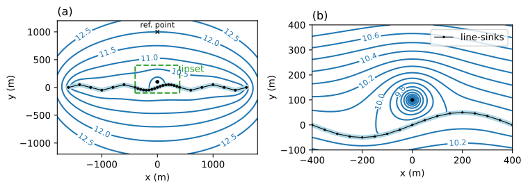
Figure 8.6 Head contours for a well near a meandering river; entire model (left) and contours near the well (right) for the green inset in the left plot.

Exercise 8.3

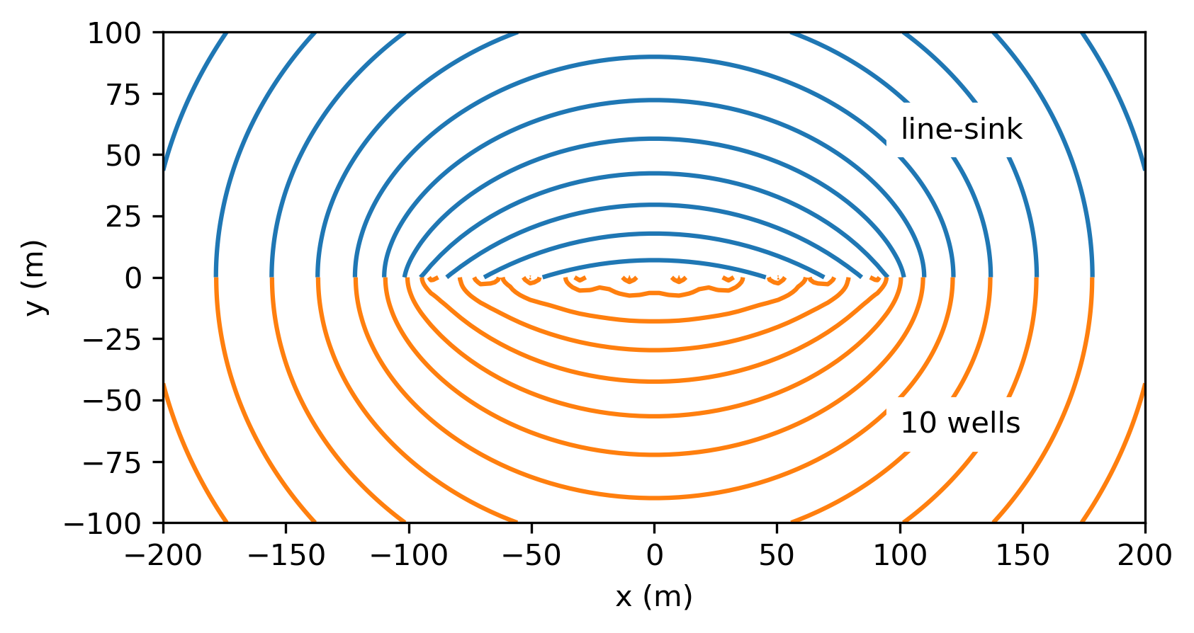
Compare a line-sink to 10 evenly spaced wells. Draw head contours for one line-sink of 200 m length and \(\sigma=2\) m\(^2\)/d. On the same plot, draw head contours for 10 evenly spaced wells with a total discharge equal to the total discharge of the line-sink. The transmissivity of the aquifer is \(T=100\) m\(^2\)/d, and the endpoints of the line-sink are at \((-100,0)\) and \((100,0)\). Specify the head to 20 m far away at \((0,10000)\).

Solution

Exercise 8.4

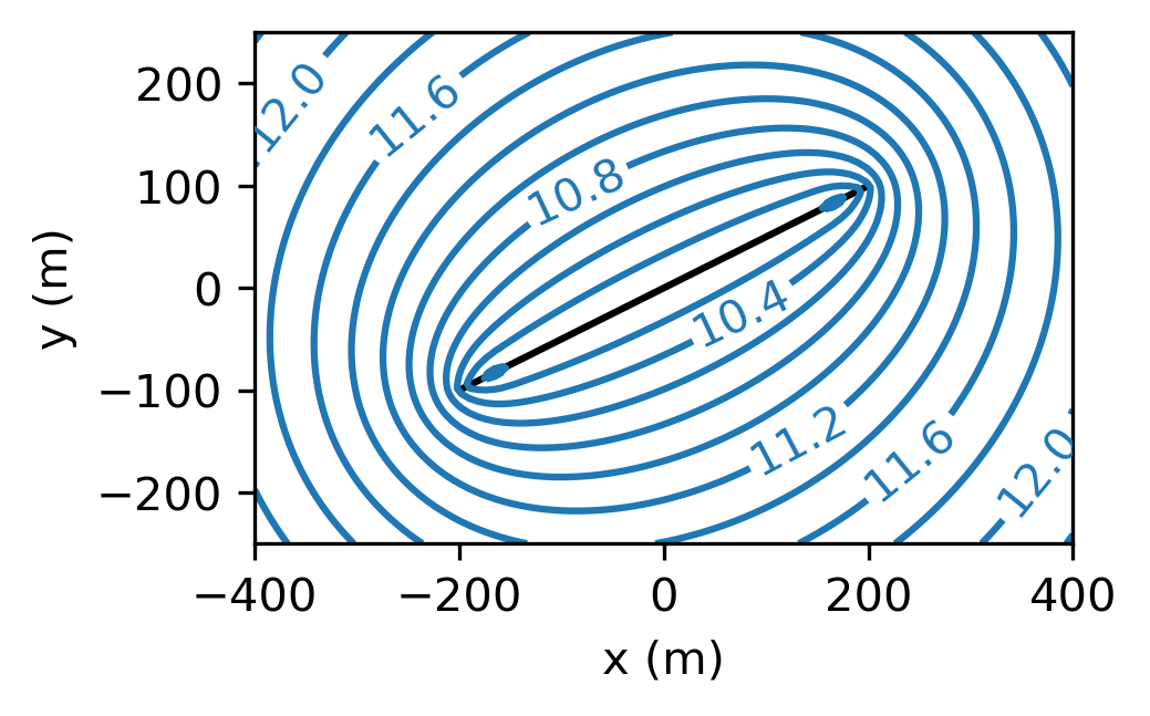
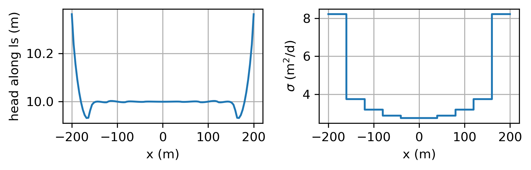
Simulate flow to a ditch with specified head of 10 m. The ditch runs from (-200, -100) till (200, 100). The head at (0,400) is 12 m. Use enough line-sinks such that the head along the ditch is approximately uniform. The transmissivity is 200 m\(^2\)/d. Plot head contours and make separate plots of the head variation along the ditch and the inflow variation along the ditch. Compute the total inflow into the ditch.

Solution

Using 11 line-sinks: \(Q = -1855\) m\(^3\)/d

Exercise 8.5

Consider a well pumping near a long and straight river along the \(x\)-axis. The transmissivity of the aquifer is 200 m\(^2\)/d and the head in the river is 8 m. The well is located at (0, 100), the well radius is 0.3 m, and the head in the well is 6 m. Simulate the river with head-specified line-sinks. Use enough line-sink of an appropriate length such that the analytic element solution is in reasonable agreement with the exact solution obtained with the method of images (Exercise 6.8). Compute the discharge of the well.

Solution

\(Q = 387\) m\(^3\)/d