3.1. Areal recharge between an impermeable boundary and a river

Consider uniform recharge at a rate \(N\) on an unconfined aquifer bounded on the left by an impermeable boundary and on the right by a river (see Figure 3.2). The problem is the same as in Section 1.3, but now the transmissivity is a function of the head \(h\) in the aquifer rather than approximated as constant. The length of the aquifer is \(L\), and the elevation of the aquifer bottom is \(z_b\). The boundary conditions are

(3.8)\[ \left. \frac{\text{d}h}{\text{d}x}\right\vert_{x=0} = 0 \]

(3.9)\[ h\vert_{x=L} = h_r \]

where \(h_r\) is the head in the river at \(x=L\).

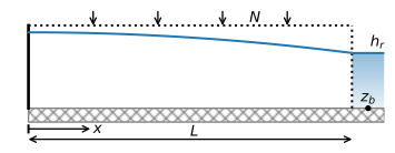
Figure 3.2 Areal recharge on an unconfined aquifer between an impermeable boundary and a river.

     The boundary conditions in terms of heads (Eqs. (3.8) and (3.9)) are converted to boundary conditions in terms of the discharge potential for unconfined flow

(3.10)\[ \left. \frac{\text{d}\Phi}{\text{d}x}\right\vert_{x=0} = 0 \]

(3.11)\[ \Phi\vert_{x=L}=\Phi_r=\tfrac{1}{2}k(h_r-z_b)^2 \]

Application of the boundary conditions to the general solution ((3.6)) gives

(3.12)\[ \Phi=-\frac{N}{2}(x^2 - L^2) + \Phi_r \]

The head is obtained from the potential with Eq. ((3.7)), which gives, using Eq. ((3.11))

(3.13)\[ h = z_b + \sqrt{2\Phi/k} = z_b + \sqrt{-N(x^2 - L^2)/k + (h_r-z_b)^2} \]

The discharge vector \(Q_x\) is obtained by differentiation of the potential as

(3.14)\[ Q_x = -\frac{\text{d}\Phi}{\text{d}x}= Nx \]

An example is presented below. The solution is compared to solution ((1.39)), where the saturated thickness was approximated as \(H=10\) m (Figure 3.3). The specific choice of the approximate \(H\) in the example leads to an underestimate of the head in the aquifer at the impermeable boundary. The discharge vector, on the other hand, is the same for both problems (compare Eqs. ((3.14)) and ((1.40))), because \(Q_x\) is independent of the choice of the approximate thickness \(H\).

# parameters
L = 1000 # aquifer length, m
H = 10 # approximate aquifer thickness used in solution of Section 1.3, m
zb = -5 # aquifer bottom, m
k = 10 # hydraulic conductivity, m/d
n = 0.3 # porosity, -
hr = 4 # specified head at the right boundary, m
N = 0.001  # areal recharge, m/d

# solution
phir = 0.5 * k * (hr - zb) ** 2
x = np.linspace(0, L, 100)
phi = -N / 2 * (x ** 2 - L ** 2) + phir
h = zb + np.sqrt(2 * phi / k)
happrox = -N / (2 * k * H) * (x ** 2 - L ** 2) + hr
Qx = N * x

# basic plot
plt.subplot(121)
plt.plot(x, h, 'C0')
plt.plot(x, happrox, 'C0--')
plt.subplot(122)
plt.plot(x, Qx, 'C1');

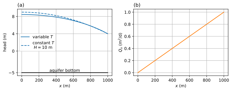
Figure 3.3 Areal recharge on an unconfined aquifer between an impermeable boundary and a river; head (left) and \(Q_x\) (right).

print(f'flux at x = 0: {-Qx[0]:.3f} m^2/d')
print(f'flux next to river at x = L: {Qx[-1]:.3f} m^2/d')

flux at x = 0: -0.000 m^2/d
flux next to river at x = L: 1.000 m^2/d

     A plot of the stream function may also be created, but now the top of the aquifer is formed by the water table (Figure 3.4).

# solution
psi = np.zeros((2, len(x)))
psi[1] = -Qx
xg = np.zeros_like(psi)
xg[:] = x
zg = np.zeros_like(psi)
zg[0] = zb
zg[1] = h

# basic streamline plot
plt.subplot(111, aspect=25)
plt.contour(xg, zg, psi, 10, colors='C1', linestyles='-')
plt.plot(x, h, 'k');

Once Loop Reflect

Figure 3.4 Streamlines in a vertical cross section for areal recharge on an unconfined aquifer between two rivers with \(\Delta\psi=0.1\) m\(^2\)/d and travel time tick marks every 2 years.

     The travel time is computed for water that reaches the water table at position \(x\) and flows to the river at \(x=L\). The horizontal component of the velocity vector is obtained as

(3.15)\[ v_x = \frac{Q_x}{n(h-z_b)} = \frac{\sqrt{Nk}}{n}\frac{x}{\sqrt{2\Phi_r/N + L^2 -x^2}} \]

The travel time can be computed, as before, as

(3.16)\[ t_\text{tr}(x, L) = \int_{x}^{L} \frac{\text{d}x}{v_x} \]

The integration is conducted analytically and gives (omitting the constant of integration)

(3.17)\[ F(x) = \int \frac{\text{d}x}{v_x} = \frac{n}{\sqrt{Nk}} \sqrt{a-x^2} - \sqrt{a} \: \text{arctanh}\left(\frac{\sqrt{a-x^2}}{\sqrt{a}}\right) \]

where

(3.18)\[ a = 2\Phi_r/N + L^2 \]

The travel time can now be computed as

(3.19)\[ t_\text{tr}(x, L) = F(L) - F(x) \]

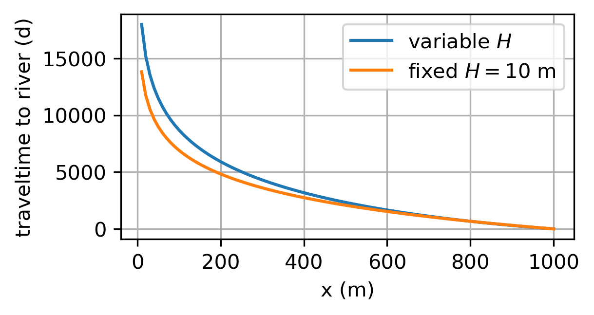
The travel time is plotted from point \(x\) to the river in Figure 3.5.

# solution
def integral(x):
    a = 2 * phir / N + L ** 2
    return np.sqrt(a - x ** 2) - np.sqrt(a) * \
           np.arctanh(np.sqrt(a - x ** 2) / np.sqrt(a))

def traveltime(x):
    return n / np.sqrt(N * k) * (integral(L) - integral(x))

x = np.linspace(10, L, 100)
trtime = traveltime(x)

# basic travel time plot
plt.plot(x, trtime);

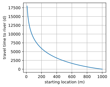
Figure 3.5 Travel time from starting location to river at \(x=L\).

Exercise 3.1

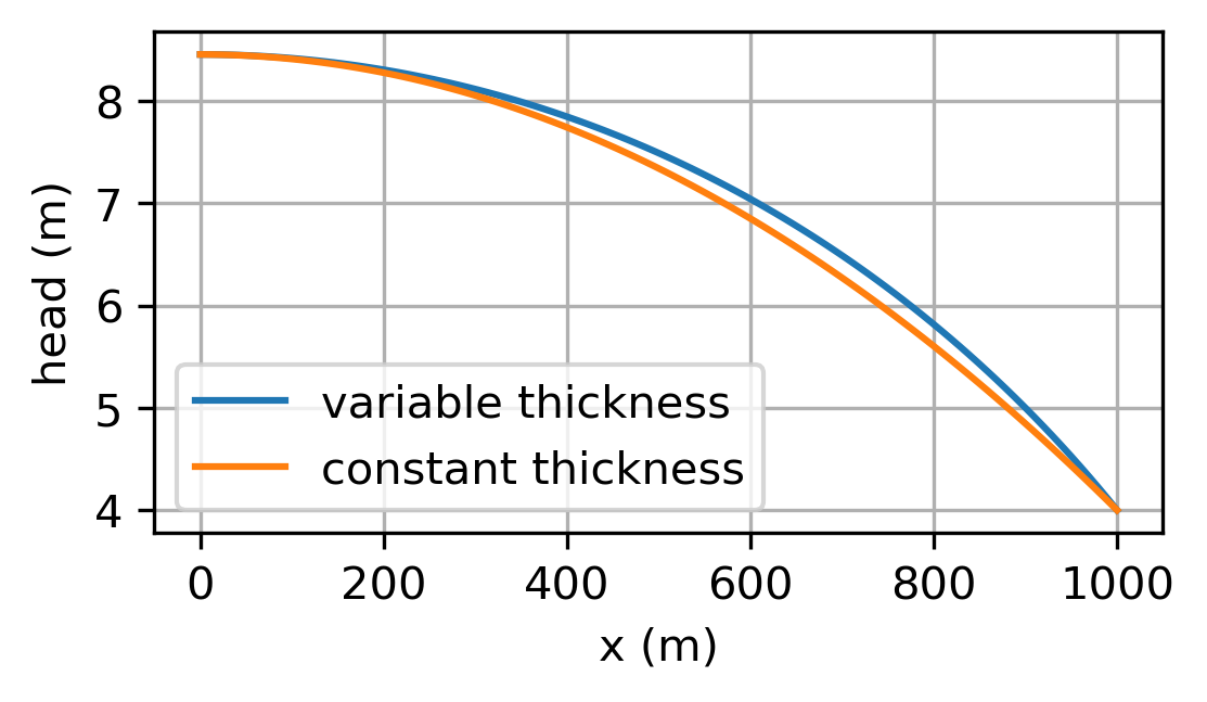
Determine the value of the effective saturated thickness \(H\) such that the head at the impermeable boundary is the same for the solutions with variable saturated thickness and constant saturated thickness. Plot the head vs. \(x\) for both solutions.

Solution

\(H = 11.227\) m

Exercise 3.2

Compare the travel time from \(x=400\) to the river computed with the analytic solution derived above and numerical integration of the integral (Eq. (3.16)) using the quad function of scipy.integrate.

Solution

\(t_\text{tr}=3182.66\) d for both

Exercise 3.3

Compute the travel time for water that recharges the aquifer at position \(x\) to reach the river at \(x=L\) for the case that the saturated thickness is approximated as constant and equal to \(H=10\) m, and add the computed travel time to Figure 3.5.

Solution

Exercise 3.4

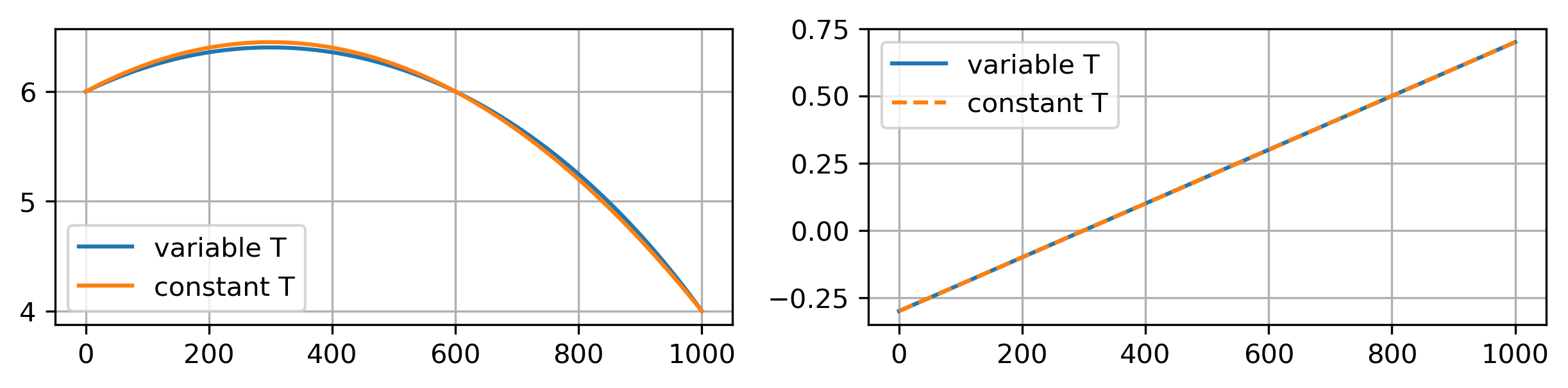
Consider the case of unconfined flow between two parallel rivers as in Section 1.2, but now the saturated thickness of the unconfined aquifer is not approximated by an effective thickness \(H\), but varies with the head instead. Compute the difference between the solution for unconfined flow with a varying saturated thickness and the solution for unconfined flow with an effective thickness \(H\). Use the parameters specified in Section 1.2. Compare the location of the water divide and the maximum head between the rivers for the two solutions.

Solution

Water divide is at same location, but the head at the water divide is slightly higher for the case with \(H=10\) m.