2.4. Flow to a river in a two-aquifer system

Many aquifers are bounded at the bottom by a leaky layer with another aquifer below. Solutions for one-dimensional steady flow in such a two-aquifer systems can be written as the sum of the solution for confined flow (Chapter 1) and the solution for semi-confined flow, as will be shown in the following.
      In what follows, the tranmissivity of the top aquifer (aquifer 0) is \(T_0\) and the transmissivity of the bottom aquifer (aquifer 1) is \(T_1\). The resistance of the leaky layer between the two aquifers is \(c\). The recharge from rainfall to the top aquifer is equal to \(N\). The vertical flow \(q_z\) through the leaky layer flow from aquifer 1 (the bottom aquifer) to aquifer 0 (the top aquifer) is

(2.33)\[ q_z = \frac{h_1 - h_0}{c} \]

where \(h_0\) and \(h_1\) are the head in the top and bottom aquifer, respectively. The head in the two-aquifer system is governed by a system of two differential equations

(2.34)\[\begin{split} \begin{split} \frac{\text{d}^2 h_0}{\text{d}x^2} & = \frac{h_0-h_1}{cT_0} - \frac{N}{T_0} \\ \frac{\text{d}^2 h_1}{\text{d}x^2} & = \frac{h_1-h_0}{cT_1} \end{split} \end{split}\]

      The solution to the system of two differential equations ((2.34)) is obtained as follows. Addition of the first differential equation multiplied by \(T_0\) and the second differential equation multiplied by \(T_1\) gives

(2.35)\[ \frac{\text{d}^2(T_0h_0 + T_1h_1)}{\text{d}x^2} = -N \]

This is Poisson’s differential equation ((1.8)), which has the general solution

(2.36)\[ T_0h_0 + T_1h_1 = \frac{-Nx^2}{2} + A'x + B' \]

where \(A'\) and \(B'\) are arbitrary constants. Subtraction of the second differential equation from the first differential equation gives, after a bit of algebra

(2.37)\[ \frac{\text{d}^2(h_0 - h_1)}{\text{d}x^2} = \frac{h_0-h_1}{\lambda^2} - \frac{N}{T_0} \]

where

(2.38)\[ \lambda=\sqrt{\frac{cT_0T_1}{T_0+T_1}} \]

This is the modified Helmholtz equation ((2.5)) with an additional constant (\(-N/T_0\)) on the right-hand side. The general solution is

(2.39)\[ h_0-h_1 = C'\text{e}^{-x/\lambda} + D'\text{e}^{x/\lambda} + \frac{N\lambda^2}{T_0} \]

where \(C'\) and \(D'\) are arbitrary constants. Expressions for \(h_0\) and \(h_1\) are obtained by combining Eqs. ((2.36)) and ((2.39)), which gives

(2.40)\[\begin{split} \begin{split} h_0 &= -\frac{N}{2T}x^2 + Ax + B + CT_1\text{e}^{-x/\lambda} + DT_1\text{e}^{x/\lambda} + \frac{T_1N\lambda^2}{T_0T} \\ h_1 &= -\frac{N}{2T}x^2 + Ax + B - CT_0\text{e}^{-x/\lambda} - DT_0\text{e}^{x/\lambda} - \frac{N\lambda^2}{T} \end{split} \end{split}\]

where \(T\) = \(T_0\) + \(T_1\) and \(A\), \(B\), \(C\), and \(D\) are parameters that must be determined from boundary conditions.

      As a first example, consider flow to a river in a two-aquifer system; areal recharge is neglected. The river is narrow and in direct contact with the the top aquifer, but not the bottom aquifer, as shown in Figure 2.11. The boundary condition at the river is

(2.41)\[ h_0|_{x=0}=h_R \]

where \(h_R\) is the river stage. Far away to the left of the river, the heads in the two aquifers are equal and the head gradient is \(\text{d}h_0/\text{d}x=\text{d}h_1/\text{d}x=G_l\), so that the discharge vector \(Q_{x_0}\) in the top aquifer is

(2.42)\[ Q_{x_0}|_{x=-\infty}=U_{l_0} = -T_0 G_l \]

and the discharge vector \(Q_{x_1}\) in the bottom aquifer is

(2.43)\[ Q_{x_1}|_{x=-\infty}=U_{l_1} = -T_1 G_l \]

The head gradient far to the right is \(G_r\) so that the discharge vector is

(2.44)\[ Q_{x_0}|_{x=\infty}=U_{r_0} = -T_0 G_r \]

and the discharge vector \(Q_{x_1}\) in the bottom aquifer is

(2.45)\[ Q_{x_1}|_{x=\infty}=U_{r_1} = -T_1 G_r \]

An amount \(\sigma\) [L\(^2\)/T] flows from the aquifer into the river per meter river normal to the plane of flow. The discharge \(\sigma\) is obtained from continuity of flow

(2.46)\[ \sigma = U_{l_0} + U_{l_1} - (U_{r_0} + U_{r_1}) \]

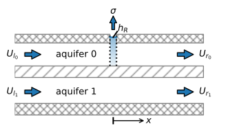
Figure 2.11 Flow to a river in a two-aquifer system.

Application of the stated boundary conditions to the general solution (2.40) gives

(2.47)\[\begin{split} \begin{split} h_0 &= -\frac{U_{l_0}}{T_0} x - \frac{T_1 \lambda}{T_0 T}\frac{\sigma}{2} \left(\text{e}^{x/\lambda} - 1\right) + h_R\\ h_1 &= -\frac{U_{l_1}}{T_1} x + \frac{\lambda }{T}\frac{\sigma}{2} \left(\text{e}^{x/\lambda} + \frac{T_1}{T_0}\right) + h_R \end{split} {\hskip 2em} x \le 0 \end{split}\]

(2.48)\[\begin{split} \begin{split} h_0 &= -\frac{U_{r_0}}{T_0} x - \frac{T_1 \lambda}{T_0 T}\frac{\sigma}{2} \left(\text{e}^{-x/\lambda} - 1\right) + h_R \\ h_1 &= -\frac{U_{r_1}}{T_1} x + \frac{\lambda }{T}\frac{\sigma}{2} \left(\text{e}^{-x/\lambda} + \frac{T_1}{T_0}\right) + h_R \end{split} {\hskip 2em} x \ge 0 \end{split}\]

The corresponding expressions for the discharge vector are

(2.49)\[\begin{split} \begin{split} Q_{x0} &= U_{l_0} + \frac{T_1}{T}\frac{\sigma}{2} \text{e}^{x/\lambda} \\ Q_{x1} &= U_{l_1} - \frac{T_1}{T}\frac{\sigma}{2} \text{e}^{x/\lambda} \end{split} {\hskip 2em} x \le 0 \end{split}\]

(2.50)\[\begin{split} \begin{split} Q_{x0} &= U_{r_0} - \frac{T_1}{T}\frac{\sigma}{2} \text{e}^{-x/\lambda} \\ Q_{x1} &= U_{r_1} + \frac{T_1}{T}\frac{\sigma}{2} \text{e}^{-x/\lambda} \end{split} {\hskip 2em} x \ge 0 \end{split}\]

The leakage factor \(\lambda\) (Eq. (2.38)) for a two-aquifer system plays the same role as for semi-confined flow: a distance \(3\lambda\) from the river, the heads and gradients in the aquifers are approximately equal.
      In the example below, the transmissivity (and hence the flow far from the river) in the bottom aquifer is twice the transmissivity of the top aquifer. Flow is towards the river from both sides, but the flow from the left is four times as large as from the right (Figure 2.12).

# parameters
k0 = 10 # hydraulic conductivity aquifer 0, m/d
k1 = 20 # hydraulic conductivity aquifer 1, m/d
H0 = 10 # thickness aquifer 0, m
H1 = 10 # thickness aquifer 1, m
Hstar = 2 # thickness leaky layer
kstar = 0.01 # hydraulic conductivity leaky layer, m/d
hR = 5 # head in river, m
Gl = -0.002 # head gradient far away to the left, -
Gr = 0.0005 # head gradient far away to the right, -

# solution
T0 = k0 * H0
T1 = k1 * H1
c = Hstar / kstar
T = T0 + T1
Ul0 = -T0 * Gl
Ul1 = -T1 * Gl
Ur0 = -T0 * Gr
Ur1 = -T1 * Gr
σ = Ul0 + Ul1 - (Ur0 + Ur1)
λ = np.sqrt(c * T0 * T1 / T)
print(f'leakage factor: {λ:.2f} m')
#
x = np.linspace(-4 * λ, 4 * λ, 401)
def hmaq(x):
    if x <= 0:
        h0 = -Ul0 / T0 * x - T1 / T0 * λ / T * σ / 2 * (np.exp(x / λ) - 1) + hR
        h1 = -Ul1 / T1 * x + λ / T * σ / 2 * (np.exp(x / λ) + T1 / T0) + hR
    else:
        h0 = -Ur0 / T0 * x - T1 / T0 * λ / T * σ / 2 * (np.exp(-x / λ) - 1) + hR
        h1 = -Ur1 / T1 * x + λ / T * σ / 2 * (np.exp(-x / λ) + T1 / T0) + hR
    return h0, h1

hmaqvec = np.vectorize(hmaq) # vectorized version of hmaq function
h0, h1 = hmaqvec(x)

def disxmaq(x):
    if x <= 0:
        Qx0 = Ul0 + T1 / T * σ / 2 * np.exp(x / λ)
        Qx1 = Ul1 - T1 / T * σ / 2 * np.exp(x / λ)
    else:
        Qx0 = Ur0 - T1 / T * σ / 2 * np.exp(-x / λ)
        Qx1 = Ur1 + T1 / T * σ / 2 * np.exp(-x / λ)
    return Qx0, Qx1

disxmaqvec = np.vectorize(disxmaq) # vectorized version of disxmaq function
Qx0, Qx1 = disxmaqvec(x)

leakage factor: 115.47 m

# basic plot
plt.subplot(121)
plt.plot(x, h0, 'C0', label='$h_0$')
plt.plot(x, h1, 'C0--', label='$h_1$')
plt.legend()
plt.subplot(122)
plt.plot(x, Qx0, 'C1', label='$Q_{x_0}$')
plt.plot(x, Qx1, 'C1--', label='$Q_{x_1}$')
plt.legend();

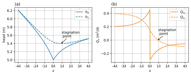
Figure 2.12 Flow to a river in a two-aquifer system; head (left) and \(Q_x\) (right).

      A contour plot of the stream function is shown in Figure 2.13. Note that part of the water coming from the left in the bottom aquifer flows past the river before it leaks to the top aquifer and flows to the river. There is a stagnation point in the bottom aquifer (\(Q_{x_1}=0\)) to the right of the river as can also be seen from the right graph of Figure 2.12.

# solution
z = [0, H1, H1 + Hstar, H1 + Hstar + H0]
psi = np.zeros((len(z), len(x)))
psi[1] = Qx1
psi[2] = Qx1
psi[3] = Qx1 + Qx0

# basic streamline plot
plt.subplot(111, aspect=10)
plt.contour(x, z, psi, np.arange(-1, 1, 0.05))
plt.axhspan(H1, H1 + Hstar, color=[.8, .8, .8]);

Figure 2.13 Streamlines in a vertical cross-section for flow to a river in the top aquifer of a two-aquifer system. Discharge between two streamlines is \(\Delta\psi=0.05\) m\(^2\)/d.

      The stated problem is fully defined by only three values: the gradients \(G_l\) and \(G_r\) far away to the left and right of the river, respectively, and the head in the river \(h_R\). \(G_l\) may be obtained from the head in one of the aquifers on the left side of the river, and \(G_r\) may be obtained from the head in one of the aquifers on the right side of the river. For example, if the head is \(h_d\) in the top aquifer at \(x=-d\), substitution in Eq. ((2.47)) gives

(2.51)\[ G_l = \frac{h_R - h_d}{d} - \frac{T_1 \lambda}{T_0 T}\frac{\sigma}{2} \frac{\left(\text{e}^{-d/\lambda} - 1\right)}{d} \]