6.2. Wells near rivers and impermeable boundaries

In the previous section, the superposition principle was applied to obtain the solution for a well pumping at the center of a circular island with recharge. Here, solutions are presented for pumping wells near a surface water boundary (e.g., river, stream, canal, or lake) and an impermeable boundary. All boundaries are approximated as long and straight; areal recharge is not simulated. Solutions for the discharge potential, the discharge vector, and the stream function are obtained through superposition and the method of images.
      The general solution for the discharge potential of well number \(n\) with discharge \(Q_n\) is obtained from the Thiem equation ((6.25)) by removing the constant part \(\Phi_R - \tfrac{Q}{2\pi}\ln(R)\) (an appropriate constant is added later depending on the boundary condition)

(6.37)\[ \Phi = \frac{Q_n}{2\pi}\ln(r_n) = \frac{Q_n}{4\pi}\ln(r_n^2) \]

where \(r_n\) is the radial distance from point \((x, y)\) to \((x_n, y_n)\), the center of well \(n\)

(6.38)\[ r_n=\sqrt{(x-x_n)^2+(y-y_n)^2} \]

The \(x\)- and \(y\)-components of the discharge vector of well \(n\) are obtained as

(6.39)\[ Q_x = -\frac{\partial\Phi}{\partial x}= -\frac{Q_n}{2\pi}\frac{x-x_n}{r_n^2} \]

(6.40)\[ Q_y = -\frac{\partial\Phi}{\partial y}=-\frac{Q_n}{2\pi}\frac{y-y_n}{r_n^2} \]

Exercise 6.4

A well is pumping at an unknown, steady rate in a confined aquifer with transmissivity \(T = 1200\) m\(^2\)/day. Near the pumping well are two observation wells. Observation well \(A\) is located 8 m from the pumping well, and observation well \(B\) is located 24 m from the pumping well. The heads in these wells are \(h_A = 134.2\) m and \(h_B = 134.3\) m. Assuming that without the well pumping there is no hydraulic gradient in the aquifer, what is the pumping rate of the well?

Solution

\(Q = 686\) m\(^3\)/d

      The stream function for a well is derived next. A single well in a homogeneous, isotropic aquifer of infinite extent results in circular equipotentials. Streamlines are straight lines to the well. As such, the stream function is a function of \(\theta\) only, where \(\theta\) is the angle measured in counterclockwise direction with respect to the positive horizontal axis in a local coordinate system centered at the well (see the left graph of Figure 6.6). The stream function for well \(n\) is

(6.41)\[ \Psi = \frac{Q_n}{2\pi}\theta_n \]

where

(6.42)\[ \theta_n=\arctan\left(\frac{y-y_n}{x-x_n}\right) \]

where \(\theta\) is measured in radians and not degrees.
      Eight streamlines are plotted in Figure 6.6. The total discharge between each two consecutive streamlines is \(Q/8\). The angle \(\theta\) is measured with respect to the positive \(x\)-axis and jumps from \(\pi\) to \(-\pi\) along the negative \(x\)-axis when going in the counterclockwise (the mathematically positive) direction. As a result, the stream function jumps across the negative \(x\)-axis, from \(Q/2\) to \(-Q/2\). This jump is unavoidable. It can be chosen differently; for example, \(\theta\) can vary from 0 to \(2\pi\), but then the stream function will jump along the positive \(x\)-axis. The line along which the stream function jumps is called the branch cut. It appears that the contouring routine plots a thicker line along the branch cut. This is because all the stream function values that are contoured fall between the values computed at the grid points just above the negative \(x\)-axis and the values computed at the grid points just below the negative \(x\)-axis. The thick line is less pronounced when more grid points are used.
      A plot with both equipotentials and streamlines is called a flow net (Figure 6.6). Equipotentials and streamlines always cross at right angles, unless the aquifer is anisotropic. It is common to use the same increments \(\Delta \Phi = \Delta \Psi\) when constructing a flow net. Note that in the code below, the angle \(\theta\) is computed with the np.arctan2 function, which computes the arctan function given a value of \(y\) and \(x\) (in that order) and returns the corresponding angle in the range \(-\pi\) to \(+\pi\). Before creating a contour plot, a subplot is created where the scale is set equal in the \(x\)- and \(y\)-directions using the aspect keyword so that, e.g., a circle indeed looks like a circle and not an ellipse.

# parameters
xw = 0 # x-location of well, m
yw = 0 # y-location of well, m
Q = 100 # discharge of well, m^3/d

# solution
xg, yg = np.meshgrid(np.linspace(-100, 100, 100), np.linspace(-100, 100, 100))
phi = Q / (4 * np.pi) * np.log(((xg - xw) ** 2 + (yg - yw) ** 2) / 100 ** 2)
psi = Q / (2 * np.pi) * np.arctan2(yg - yw, xg - xw)

# basic flow net (right graph)
plt.subplot(111, aspect=1)
plt.contour(xg, yg, psi, np.arange(-Q / 2, Q / 2, Q / 8))
plt.contour(xg, yg, phi, np.arange(phi.min(), phi.max(), Q / 8));

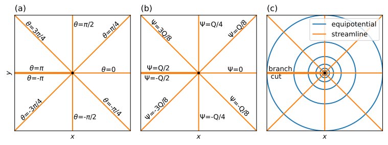
Figure 6.6 Angle \(\theta\) measured in a local coordinate system centered at the well (left), stream function along eight streamlines including branch cut (middle), and flow net (right) for radial flow to a well.

      As an example of the superposition principle, consider the case of an extraction well and an injection well, also referred to as a well doublet. Well 0 is located at \((x_0,y_0)=(-d,0)\) and extracts with discharge \(Q_0 = Q\). Well 1 is located at \((x_1,y_1)=(d,0)\) and has an injection rate that is equal in magnitude to the discharge of well 0, which means that \(Q_1=-Q\). The head at \((x,y)=(0,0)\) is equal to \(h_c\), which is converted to a discharge potential \(\Phi_c\). The solution is obtained by the addition of two solutions ((6.37)) as (recall that \(\ln(r_0^2) - \ln(r_1^2) = \ln(r_0^2 / r_1^2)\))

(6.43)\[ \Phi = \frac{Q}{4\pi}\ln(r_0^2 / r_1^2) + \Phi_c \]

where \(r_0\) and \(r_1\) are the distances to well 0 and well 1, respectively. Note that at \((x,y)=(0,0)\), \(r_0 = r_1\) so that the potential is indeed equal to \(\Phi_c\). Expressions for the discharge vector and the stream function are obtained in a similar fashion through superposition. A flow net and a streamplot are shown below. All water that is injected by the right well of the doublet flows to the left well of the doublet although the path may be very long. The branch cut in the stream function only extends from the injection well to the extraction well (left graph of Figure 6.7). To the left of the pumping well (\(x\le -d\)), the branch cut of the pumping well cancels the branch cut of the injection well.

# parameters
T = 100 # transmissivity, m^2/d
hc = 0 # head at (0, 0)
d = 100 # half distance between the two wells, m
Q = [100, -100] # discharges of wells, m^3/d
xw = [-d, d] # x-locations of wells, m
yw = [0, 0] # y-locations of wells, m
phic = T * hc # discharge potential at origin, m^3/d

# solution
xg, yg = np.meshgrid(np.linspace(-200, 200, 100), np.linspace(-150, 150, 100))
pot = phic
psi = 0.0
Qx = 0.0
Qy = 0.0
for n in range(2):
    rsq = (xg - xw[n]) ** 2 + (yg - yw[n]) ** 2
    pot += Q[n] / (4 * np.pi) * np.log(rsq)
    psi += Q[n] / (2 * np.pi) * np.arctan2(yg - yw[n], xg - xw[n])
    Qx += -Q[n] / (2 * np.pi) * (xg - xw[n]) / rsq
    Qy += -Q[n] / (2 * np.pi) * (yg - yw[n]) / rsq

# basic plot
plt.figure(figsize=(8, 4))
plt.subplot(121, aspect=1)
plt.contour(xg, yg, pot, np.arange(phic - 100, phic + 100, 10))
plt.contour(xg, yg, psi, np.arange(-Q[0], Q[0], 10))
plt.subplot(122, aspect=1)
plt.streamplot(xg, yg, Qx, Qy);

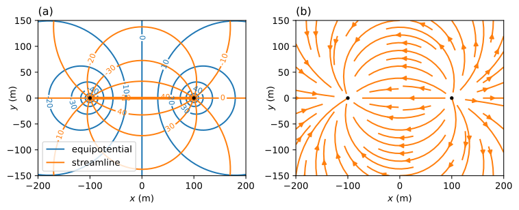
Figure 6.7 Flow net (left) and streamplot (right) for a well doublet.

      Interestingly, the potential is constant and equal to \(\Phi_c\) along the entire line \(x = 0\). This makes sense by looking at Eq. ((6.43)). After all, everywhere along the line \(x = 0\), the distance to well 0 is equal to the distance to well 1 so that \(\ln(r_0^2/r_1^2)=0\). This means that the left half of the flow field shown in Figure 6.7 \((x\le 0)\) represents the solution for a well pumping near a long and straight river with \(\Phi=\Phi_c\) along \(x = 0\). This method of obtaining the solution for a well near a river with constant head is known as the method of images.

Exercise 6.5

A well is located 65 m from a river that is roughly straight near the well. The well is installed in a 0.8-m-diameter hole. The well screen and the river are in direct contact with the same aquifer, which has an estimated transmissivity \(T = 150\) m\(^2\)/day. The well has been pumping for a long time at a rate of \(Q = 600\) m\(^3\)/day. Estimate the head in the well using the river level as the datum.

Solution

\(h_w = -3.68\) m

Exercise 6.6

For the example above, compute the stream function at \((x,y)=(0,100)\), \((x,y)=(0,\varepsilon)\), \((x,y)=(0,-\varepsilon)\), \((x,y)=(0,-100)\), where \(\varepsilon\) is a small increment, by determining the appropriate angles, and compare the answer to results with the arctan2 function.

Solution

\(\Psi = [-25, -50, 50, 25]\) m\(^3\)/d

      The method of images is an application of the superposition principle. Wells (or other singularities) are placed outside of the problem domain, and symmetry is used to satisfy conditions specified along boundaries. A well near a river with constant head is simulated by adding an image well on the other side of the river. The discharge of the image well must be equal, but opposite in sign to the discharge of the well, and the image well must be located at the “image location” of the well, that is, the same distance from the river, but on the other side. The solution for multiple wells near a river may be obtained in the same fashion, as long as a corresponding image well is added for each well.
      A well near an impermeable rock formation (an impermeable or no-flow boundary) may be simulated by adding an image well with the same discharge on the other side of the impermeable boundary. An example of a well near an impermeable boundary along \(x = 0\) is shown in Figure 6.8. The code for the solution and basic plot is the same as the code above, and is not repeated. Only the values of the discharge Q are changed.

# changed parameters
Q = [100, 100] # discharge of well and image well, m^3/d

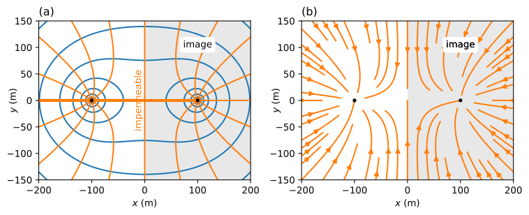
Figure 6.8 Flow net (left) and streamplot (right) for a well near an impermeable boundary.

      As a final example of the method of images, consider flow to a well near a river with a head-specified boundary (constant discharge potential \(\Phi=\Phi_c\)) along the negative \(x\)-axis and an impermeable boundary along the negative \(y\)-axis (Figure 6.9). The well has discharge \(Q\) and is located at \((x_0,y_0)\), where both \(x_0\) and \(y_0\) are negative. The solution for this problem requires three image wells. First, an image well with discharge \(Q\) is placed at \((-x_0,y_0)\), which ensures that the negative \(y\)-axis is an impermeable boundary. Next, image wells with discharge \(−Q\) are placed at \((x_0,-y_0)\) and \((-x_0,-y_0)\) so that the negative \(x\)-axis is a specified head boundary, while the negative \(y\)-axis remains an impermeable boundary. The location and discharge of the well and three image wells are shown in the left side of Figure 6.9. The discharge potential may be written as

(6.44)\[ \Phi = \frac{Q}{2\pi}\ln\left(\frac{r_0 r_1}{r_2r_3}\right) + \Phi_c \]

It is easy to verify that everywhere along the river (specified head) \(r_0=r_2\) and \(r_1=r_3\) so that, indeed, the potential (and hence the head) is constant. The boundary condition along the impermeable boundary may be verified by writing out an equation for \(Q_x\). A flow net for the flow domain is created below. The code below creates a flow net with a pretty ugly branch cut along the line \(y = −50\). This branch cut is not shown in Figure 6.9 by separately contouring the domain from \(y = −150\) to just below \(y = −50\) and then, on the same graph, from just above \(y = −50\) to \(y = 0\) (code is not shown).

# parameters
xw = [-100, 100, -100, 100] # x-locations of well and image wells, m
yw = [-50, -50, 50, 50] # y-locations of well and image wells, m
Qw = [100, 100, -100, -100] # discharge of well and image wells, m^3/d

# solution
xg, yg = np.meshgrid(np.linspace(-200, 0, 101), np.linspace(-150, 0, 101))
phi = 0
psi = 0
for n in range(4):
    phi += Qw[n] / (4 * np.pi) * np.log((xg - xw[n]) ** 2 + (yg - yw[n]) ** 2)
    psi += Qw[n] / (2 * np.pi) * np.arctan2(yg - yw[n], xg - xw[n])

# flow net in right graph
plt.subplot(111, aspect=1)
plt.contour(xg, yg, phi, np.arange(-100, 100, 5), colors='C0')
plt.contour(xg, yg, psi, np.arange(-200, 200, 5), colors='C1');

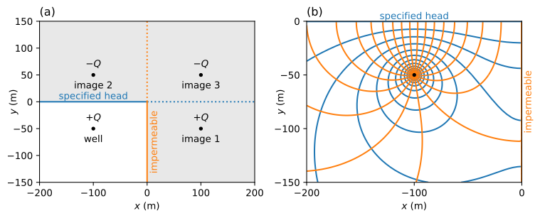
Figure 6.9 Layout of well and image wells (left) and flow net of the flow domain (right) for a well near a specified-head boundary and an impermeable boundary.

      Many analytical solutions for problems with wells and equipotential boundaries and/or impermeable boundaries may be obtained by the method of images. The method of images works for many types of flow, including confined flow, unconfined flow, interface flow, semi-confined flow, and transient flow, and is also applicable to some problems with a Robin boundary condition or an inhomogeneity boundary.

Exercise 6.7

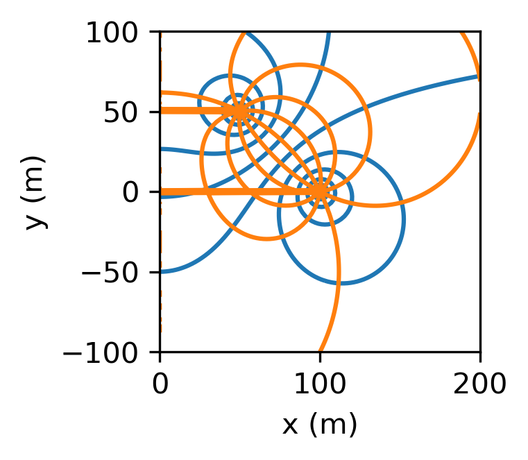
A doublet of a well and an injection well are located near an impermeable boundary located along the \(y\)-axis; the radius of both wells is 0.3 m. The extraction well is located at \((x, y) = (100, 0)\) and has a discharge \(Q = 100\) m\(^3\)/d, and the injection well is located at \((x, y) = (50, 50)\) and has an injection rate 100 m\(^3\)/d. The aquifer is confined with transmissivity \(T = 80\) m\(^2\)/d. Far away from the doublet, the head in the aquifer is zero. Draw a flow net, and compute the heads at the wells.

Solution

\(h = -1.04\) m at extraction well
\(h = 1.18\) m at injection well

Exercise 6.8

A well is located a distance \(d = 50\) m from a long and straight river with water level \(h_r = 20\) m. The river is in direct contact with the aquifer, and the radius of the well is 0.3 m. The transmissivity of the aquifer may be approximated as constant and equal to \(T = 200\) m\(^2\)/d. Compute the discharge of the well such that the head at the well is 2 m below the water level in the river.

Solution

\(Q = 432.6\) m\(^3\)/d

Exercise 6.9

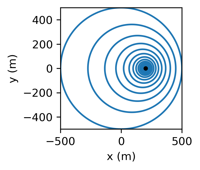
Consider a well pumping with discharge \(Q\) on a circular island with radius \(R\); the radius of the well is \(r_w\). The origin of the coordinate system is at the center of the island, and the well is located at \((x, y) = (d, 0)\). The head at the edge of the island is \(h_0\). The transmissivity of the aquifer may be approximated as constant and equal to \(T\). An expression for the head on the island may be obtained with the method of images for a circle (Strack, 1989).

(6.45)\[ h = \frac{Q}{4\pi T} \ln\left[\frac{(x-d)^2 + y^2}{(x - R^2/d)^2 + y^2} \frac{R^2}{d^2}\right] + h_0 \]

Compute and draw head contours, and compute the head at the well. Given: \(T = 200\) m\(^2\)/d, \(R = 500\), m, \(d = 200\) m, \(Q = 500\) m\(^3\)/d, \(r_w = 0.3\) m, and \(h_0 = 10\) m.

Solution

\(h_w = 7.12\) m