10.4. Spatially varying head at the top of the aquifer

The water table in an unconfined aquifer is sometimes very roughly approximated as a subdued replica of the topographic surface. This makes some intuitive sense, because groundwater may discharge at a low point in the landscape. Groundwater that recharges below the topographic highs has to take a relatively long path to the discharge area in the valley, which necessitates a hydraulic head gradient, and thus a mounding of the water table. It turns out, however, that the water table and the topographic surface are poorly correlated or even uncorrelated in many unconfined aquifers (Haitjema and Mitchell-Bruker, 2005). Nonetheless, an undulating water table may be a useful approximation to conceptualize regional flow patterns.
      In this section, flow systems are investigated where the head at the top of the aquifer is specified to consist of one or more sinusoidal functions, approximating a subdued sequence of topographic highs and lows. The problem is discussed here because it resembles the famous solution of Tóth (1963), which is often used to investigate nested flow domains in basin-scale models. As this is a problem where the head is specified at the top of the aquifer, it must be verified that the resulting flow through the top of the aquifer is hydrologically realistic.

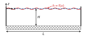
Figure 10.13 Vertical aquifer cross section in which flow is driven by a specified head at the top of the aquifer.

      Consider steady two-dimensional flow in the vertical plane (Figure 10.13). The hydraulic conductivity is \(k\) and the bottom of the aquifer is horizontal at \(z=-H\). The aquifer is a distance \(L\) long and the thickness of the aquifer is approximated as constant and equal to \(H\). Flow is governed by Laplace’s equation ((10.4)). The lateral boundaries and the base of the aquifer are impermeable

(10.36)\[ q_x|_{x=0, z} = q_x|_{x=L, z} = q_z|_{x, z=-H} = 0 \]

The head \(h\) at the top of the aquifer is specified to vary periodically as a cosine with amplitude \(a\) and period \(p=2L/n\), where \(n\) is an arbitrary integer

(10.37)\[ h|_{x,z=0} = a \cos(2\pi x/p) \]

In terms of the specific discharge potential, the boundary conditions are

(10.38)\[ \left.\frac{\partial \phi}{\partial x}\right|_{x=0, z} = \left.\frac{\partial \phi}{\partial x}\right|_{x=L, z} = \left.\frac{\partial \phi}{\partial z}\right|_{x, z=-H} = 0 \]

and

(10.39)\[ \phi|_{x,z=0} = A \cos(2\pi x/p) \]

where \(A=ka\).
      The solution for the specific discharge potential is obtained from separation of variables as (e.g., Craig, 2008)

(10.40)\[ \phi = \frac{A\cos(2\pi x/p)\cosh[2 \pi (z + H)/ p]}{\cosh(2 \pi H / p)} \]

The corresponding complex potential is

(10.41)\[ \omega = A \frac{\cos[2 \pi (\zeta + Hi) / p]}{\cosh(2 \pi H / p)} \]

where \(\zeta=x + iz\). The complex specific discharge is obtained as

(10.42)\[ q_x - iq_z = -\frac{\text{d} \omega}{\text{d}\zeta} = \frac{2\pi A}{p} \frac{\sin[2 \pi (\zeta + Hi) / p]}{\cosh(2 \pi H / p)} \]

The vertical flux at the top of the aquifer is a cosine function, just like the head

(10.43)\[ q_z = \frac{-2\pi A}{p}\frac{\cos(2\pi x/p)\sinh[2\pi(z+H)/p]}{\cosh(2\pi H/p)} \]

      As a first example, consider the case where the head at the top of the aquifer is a sequence of two highs and two lows, starting with a high of 0.2 m on the left and ending with a low of -0.2 m on the right. The head specified at the top of the aquifer, the resulting vertical flux at the top of the aquifer, and the resulting flow net are plotted in Figure 10.14. The resulting flow field has three local flow cells: water flows from the highs to the lows. All three flow cells are identical. As the head is specified at the top of the aquifer, it must be checked whether the vertical flux at the top of the aquifer (i.e., the recharge) is hydrologically possible. For the given parameters, the highest vertical flux at the top of the aquifer is \(\sim 1.5\) mm/d, which can be possible from precipitation in many climates. The flow net for the same situation, but with a ten times higher hydraulic conductivity, looks exactly the same, but the highest vertical flux at the top of the aquifer is also 10 times higher. This requires a recharge of 15 mm/d, which seems unrealistic except maybe for the wettest regions on the planet.

# parameters
k = 1 # hydraulic conductivity, m/d
L = 1200 # length of aquifer, m
H = 200 # thickness of aquifer, m
a = 0.2 # amplitude of head variation, m
p = 2 * L / 3 # period of head variation, m
A = k * a # amplitude of potential variation, m^2/d

# solution
def omega(x, z, H, A, p):
    zeta = x + 1j * z
    return A * np.cos(2 * np.pi * (zeta + H * 1j) / p) / \
               np.cosh(2 * np.pi * H / p)

def discomplex(x, z, H, A, p):
    zeta = x + 1j * z
    return 2 * np.pi * A / p * np.sin(2 * np.pi * (zeta + H * 1j) / p) / \
                               np.cosh(2 * np.pi * H / p)

xg, zg = np.meshgrid(np.linspace(0, L, 100), np.linspace(-H, 0, 100))
om = omega(xg, zg, H, A, p)
wdis = discomplex(xg, zg, H, A, p)
htop = om.real[-1] / k
qtop = -wdis.imag[-1]

# basic plot h, qz, flownet, sharing the x-axis
fig, ax = plt.subplots(3, 1, sharex=True, squeeze=True, 
                       gridspec_kw={'height_ratios':[1, 1, 2]})
plt.sca(ax[0])
plt.plot(xg[0], htop)
plt.sca(ax[1])
plt.plot(xg[0], qtop * 1000)
plt.sca(ax[2])
plt.contour(xg, zg, om.real / k, np.arange(-0.2, 0.21, 0.02))
plt.contour(xg, zg, om.imag, np.arange(-0.2, 0.21, 0.02))
plt.axis('scaled');

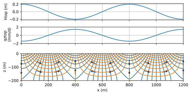
Figure 10.14 Flow caused by periodically varying specified head at the top of the aquifer (top), the resulting vertical flow at the top of the aquifer (middle), and the resulting flow net with \(\Delta h=2\) cm and \(\Delta \psi=0.02\) m\(^2\)/d (bottom).

      The flow in one flow cell is compared to the flow obtained with a Dupuit model for the same situation. The Dupuit solution for the head is simple, as it is equal to the boundary condition at the top of the aquifer (Eq. (10.37))

(10.44)\[ h = a \cos(2\pi x/p) \]

The corresponding expression for the Dupuit discharge vector is

(10.45)\[ Q_x = \frac{kHa2\pi}{p}\sin(2\pi x/p) \]

For the two-dimensional solution, the vertically integrated flow in the aquifer is equal to minus the stream function at the top of the aquifer. The two-dimensional solution is compared to the Dupuit solution for the case that there is one flow cell in the 1200 m long domain; the Dupuit solution is a reasonable approximation for a flow cell that is 1200 m long and 200 m deep (Figure 10.15). For the case that there are three flow cells in the domain (as in Figure 10.14), the Dupuit solution is a poor approximation as one flow cell is 400 m long and 200 m deep, which is far from predominantly horizontal.

# solution for flow cell of 1200 m
L = 1200
p = 2 * L # one flow cell
x = np.linspace(0, L, 100)
Qx2D = -omega(x, 0, H, A, p).imag # Qx2D = -psi
QxDupuit = k * H * a * 2 * np.pi / p * np.sin(2 * np.pi * x / p)
# grid of stream function
xg, zg = np.meshgrid(np.linspace(0, L, 400), np.linspace(-H, 0, 100))
psi2D = omega(xg, zg, H, A, p).imag
xd = xg[0]
zd = [-H, 0]
psiDupuit = np.zeros((2, len(xd)))
psiDupuit[1] = -k * H * a * 2 * np.pi / p * np.sin(2 * np.pi * xd / p)

# basic plot
plt.subplot(211)
plt.plot(x, Qx2D, label='2D solution')
plt.plot(x, QxDupuit, label='Dupuit solution')
plt.legend()
plt.subplot(212, aspect=1)
plt.contour(xg, zg, psi2D, np.arange(-0.2, 0, 0.02), colors='C1')
plt.contour(xd, zd, psiDupuit, np.arange(-0.2, 0, 0.02), colors='C0');

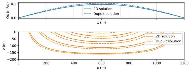
Figure 10.15 Comparision of two-dimensional flow solution to Dupuit solution for one flow cell of 1200 m length; \(Q_x\) (top) and streamlines (bottom).

     The head fluctuation at the top of the aquifer can be an arbitrary combination of cosine functions (Eq. (10.37)) with different amplitudes and different periods. For example, it is possible to approximate the head a the top of the aquifer with a constant slope \(-\Delta h / L\) by a Fourier series plus a constant

(10.46)\[ -\Delta h \frac{x}{L} \approx -\frac{\Delta h}{2} + \Delta h\sum_{n=1,3,5,...}^\infty \frac{4}{n^2\pi^2}\cos\left(\frac{n\pi x}{L}\right) \]

As an example, the flow problem is solved for the case that the head at the top of the aquifer consists of a constant slope plus one periodic variation

(10.47)\[ h|_{x,z=0}=-\Delta h \frac{x}{L} + a \cos(2\pi x/p) \]

The resulting flow net (Figure 10.16) consists of three local flow cells and one regional flow cell where water that infiltrates on the left exfiltrates all the way to the right of the aquifer, flowing below the local flow cells. The regional flow cell only occurs when the aquifer is deep enough. Note that it is again questionable whether the resulting vertical flux at the top of the aquifer is hydrologically possible, as is explored in the exercises.

# additional parameters and changed parameters
delh = 2 # head drop over distance L, m
p = L / 3 # period of head varation, m
nterms = 100 # number of terms in Fourier series

# solution
xg, zg = np.meshgrid(np.linspace(0, L, 200), np.linspace(-H, 0, 200))
om = np.zeros(xg.shape, dtype='complex')
om -= 0.5 * delh
for n in range(1, nterms + 1, 2):
    A = 4 * k * delh / (n ** 2 * np.pi ** 2)
    om += omega(xg, zg, H, A, 2 * L / n)
om += omega(xg, zg, H, k * a, p)
htop = om.real[-1] / k

# basic flownet
plt.subplot(111, aspect=1)
plt.contour(xg, zg, om.real, 10, colors='C0')
plt.contour(xg, zg, om.imag, 10, colors='C1');

Figure 10.16 Flow caused by a specified head at the top of the aquifer consisting of a constant slope \(\Delta h/ L\) and a periodically varying specified head; specified head (top) and resulting flow net (bottom).

Exercise 10.5

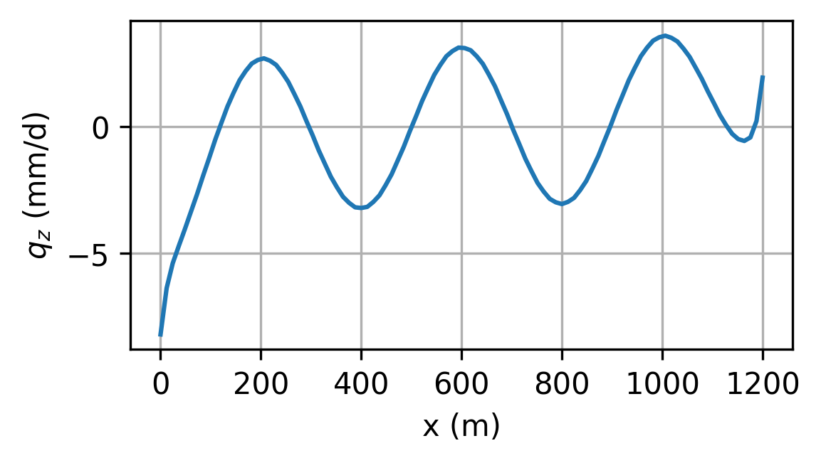
Compute and plot \(q_z\) at the top of the aquifer for the example of Figure 10.5 with \(\Delta h=2\) m.

Solution

Exercise 10.6

Create flow nets for three different aquifer thicknesses: \(H=70\) m, \(H=90\) m, and \(H=110\) m, and determine for which of these aquifer thicknesses there are no regional flow cells.

Solution

No regional flow cell for \(H=70\) m, because \(q_x=0\) between local flow cells along the bottom of the aquifer.