6.3. Wells near an inhomogeneity boundary

Hydraulic properties always vary at least a little bit throughout an aquifer. A common approach to representing varying aquifer properties is to divide the aquifer up into zones of different, but homogeneous properties; each zone is referred to as an inhomogeneity. Inside an inhomogeneity, the hydraulic conductivity, base elevation, and/or thickness of the aquifer may be different from its surroundings. As such, the transmissivity of the aquifer is referred to as piecewise constant.
      The boundary conditions at the inhomogeneity boundary are that both the head and the normal component of flow are continuous across it. As a result, the component of flow parallel to the inhomogeneity boundary jumps. This is a direct consequence of the condition that the head is continuous. For example, consider an inhomogeneity boundary along the \(y\)-axis, as shown in Figure 6.10. The transmissivity to the left of the boundary is \(T_L\), and the transmissivity to the right of the boundary is \(T_R\). The head is the same on either side of the inhomogeneity boundary, which means that also the head gradient \(\partial h/\partial y\) is continuous across the boundary. As a result, the component of the discharge vector parallel to the boundary, in this case \(Q_y\), is \(Q_y^-=-T_L\partial h/\partial y\) on the left side of the boundary and \(Q_y^+=-T_R\partial h/\partial y\) on the right side of the boundary. The jump in the component of flow parallel to the inhomogeneity boundary is referred to as a shear flow.
      The direction of a streamline changes abruptly when it crosses an inhomogeneity boundary. This is a direct consequence of the shear flow along the boundary. For example, consider one point on the inhomogeneity boundary along the \(y\)-axis of Figure 6.10. The flow just to the left of the boundary is \((Q_x^-, Q_y^-)\), and the flow just to the right of the boundary is \((Q_x^+, Q_y^+)\). The angle \(\theta^-\) between \(\vec{Q}^-\) and the normal to the boundary is

(6.46)\[ \tan(\theta^-) = Q_y^-/Q_x^- \]

Similarly, the angle \(\theta^+\) between \(\vec{Q}^+\) and the normal to the boundary is

(6.47)\[ \tan(\theta^+) = Q_y^+/Q_x^+ \]

Since \(Q_x^-=Q_x^+\), this gives

(6.48)\[ \frac{\tan(\theta^-)}{\tan(\theta^+)} = \frac{T_L}{T_R} \]

This means that when water flows from higher transmissivity to lower transmissivity (\(T_R<T_L\), as shown in Figure 6.10), the angle between the discharge vector and the normal to the boundary decreases. It is said that the discharge vector is refracted toward the normal.

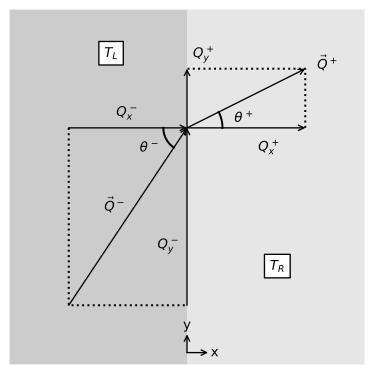
Figure 6.10 Refraction of the discharge vector at an inhomogeneity boundary for the case that \(T_R<T_L\).

      As an example, consider a well pumping near an inhomogeneity boundary along the \(y\)-axis, as discussed above. The well is located at \((x, y) = (−d, 0)\) and is numbered well 0. The solution for an inhomogeneity boundary is obtained with the method of images by placing an image well at \((x, y) = (d, 0)\) and choosing the discharge of the image well such that the boundary conditions along the inhomogeneity boundary are met. The solution for the head is (e.g., Strack, 2017, Section 8.10)

(6.49)\[ h = \frac{Q}{2\pi T_L}\ln\left(\frac{r_0}{r_1}\right) + \frac{Q}{\pi(T_L + T_R)}\ln\left(\frac{r_1}{R}\right) {\hskip 2em} x\le 0 \]

(6.50)\[ h = \frac{Q}{\pi(T_L + T_R)} \ln\left(\frac{r_0}{R}\right) {\hskip 2em} x\ge 0 \]

where \(r_0=\sqrt{(x+d)^2 + y^2}\), \(r_1 = \sqrt{(x-d)^2 + y^2}\), and the head is set to zero at \((x,y)=(0,\sqrt{R^2-d^2})\). The solution for the stream function is

(6.51)\[ \Psi = \frac{Q}{2\pi}(\theta_0 - \theta_1) + \frac{QT_L}{\pi(T_L + T_R)}\theta_1 {\hskip 2em} x\le 0 \]

(6.52)\[ \Psi = \frac{QT_R}{\pi(T_L + T_R)} \theta_0 {\hskip 2em} x\ge 0 \]

where \(\theta_0=\arctan(y/(x+d))\) and \(\theta_1=\arctan(-y/(d-x))\). Note that \(\theta_0\) varies from \(-\pi\) to \(\pi\) while \(\theta_1\) varies from 0 to \(2\pi\).
      An example is shown where \(T_R\) varies from \(T_L / 5\) to \(5 T_L\) (Figure 6.11). The total discharge that the well pumps from the zone on the right, where \(T = T_R\), is \(T_R Q / (T_L + T_R)\). For the case that \(T_R\) is small relative to \(T_L\), the inhomogeneity boundary starts to represent an impermeable boundary. For the case that \(T_R\) is large relative to \(T_L\), the inhomogeneity boundary starts to represent an equipotential. Curiously, for this case of a well pumping near a straight inhomogeneity boundary, the streamlines on the right side of the inhomogeneity boundary are straight and directed toward the well.

# parameters
d = 100 # distance of well from inhomogeneity boundary, m
Q = 100 # discharge of well, m^3/d
TL = 100 # transmissivity on left side, m^2/d

def head_and_psi(x, y, TL, TR, d=100, Q=100):
    R = 1000
    r0 = np.sqrt((x + d) ** 2 + y ** 2)
    r1 = np.sqrt((x - d) ** 2 + y ** 2)
    theta0 = np.arctan2(y, x + d)
    theta1 = np.arctan2(-y, d - x)
    if x < 0:
        h = Q / (2 * np.pi * TL) * np.log(r0 / r1) + \
            Q / (np.pi * (TL + TR)) * np.log(r1 / R) 
        psi = Q / (2 * np.pi) * (theta0 - theta1) + \
            Q * TL / (np.pi * (TL + TR)) * theta1
    else:
        h = Q / (np.pi * (TL + TR)) * np.log(r0 / R)
        psi = Q * TR / (np.pi * (TL + TR)) * theta0
    return h, psi

hpsifunc = np.vectorize(head_and_psi)

xg, yg = np.meshgrid(np.linspace(-200, 200, 100), np.linspace(-150, 150, 100))
h, psi = hpsifunc(xg, yg, TL=TL, TR=TL / 5, d=d, Q=Q)
h_0, psi_0 = hpsifunc(xg[0, :], 0, TL=TL, TR=TL / 5, d=d, Q=Q)

# basic plot
plt.subplot(121, aspect=1, title='$T_L$=100 m$^2$/d, $T_R$=20 m$^2$/d')
plt.contour(xg, yg, h, 40, colors='C0')
plt.contour(xg, yg, psi, np.arange(-50, 50, 2.5), colors='C1')
plt.axvspan(0, 200, color=[.9, .9, .9])
plt.subplot(122, title='$T_L$=100 m$^2$/d, $T_R$=20 m$^2$/d')
plt.plot(xg[0, :], h_0, 'C0', label='y=0 m')
plt.axvspan(0, 200, color=[.9, .9, .9]);

Figure 6.11 Pumping well near an inhomogeneity boundary; contour plot (left) with a contour interval of \(Q/40\), and head along \(y = 0\) (right).