3. Steady one-dimensional unconfined flow with variable saturated thickness

In the previous chapters, the saturated thickness of the aquifer was approximated as constant. The approximation of a constant saturated thickness gives reasonable results when the variation of the saturated thickness is not too large. In this chapter, solutions are derived for unconfined flow with a saturated thickness that varies with the head. The Dupuit–Forchheimer approximation is adopted so that the head is equal to the elevation of the water table and the horizontal flow is distributed uniformly over the saturated thickness (Figure 3.1).

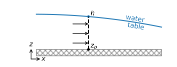
Figure 3.1 Unconfined Dupuit–Forchheimer flow over a horizontal base.

     The elevation of the base of the aquifer is denoted as \(z_b\), so that the saturated thickness is equal to \(h-z_b\) (Figure 3.1) and the discharge vector can be written as

(3.1)\[ Q_x=-k(h-z_b)\frac{\text{d}h}{\text{d}x}=-\frac{\text{d}}{\text{d}x}\left(\tfrac{1}{2}k(h-z_b)^2\right) \]

where it is used that the elevation of the base of the aquifer and the hydraulic conductivity are constant.
     While it is possible to obtain a solution for unconfined flow in terms of the head \(h\), it is more convenient to solve unconfined flow problems using a discharge potential. The discharge potential for unconfined flow \(\Phi\) is introduced as

(3.2)\[ \Phi = \tfrac{1}{2}k(h-z_b)^2 \]

so that the discharge vector can be written as

(3.3)\[ Q_x = -\frac{\text{d}\Phi}{\text{d}x} \]

Flow fields where the discharge vector \(Q_x\) may be written as minus the derivative of a discharge potential are referred to as potential flow. Potential flow solutions exist in many fields, including fluid mechanics and heat transport.
     Discharge potentials are an abstract quantity that cannot be measured in the field. Groundwater problems are, of course, not formulated in terms of discharge potentials, but in terms of heads. To be able to use a potential solution, boundary conditions in terms of heads must be converted to boundary conditions in terms of discharge potentials. After a potential solution is evaluated, the computed potential must be converted back to a head. The use of discharge potentials makes it possible to solve fairly complicated problems, including unconfined flow and interface flow in coastal aquifers (Chapter 4).
     The continuity equation for one-dimensional flow is still Eq. ((1.5))

(3.4)\[ \frac{\text{d}Q_x}{\text{d}x}=N \]

Substitution of Eq. ((3.3)) for \(Q_x\) into the continuity equation gives

(3.5)\[ \frac{\text{d}^2\Phi}{\text{d}x^2}=-N \]

The general solution to this second order ordinary differential equation may be written as

(3.6)\[ \Phi=-\frac{N}{2}x^2 + Ax +B \]

where the constants \(A\) and \(B\) need to be determined from the boundary conditions. Once a solution for the discharge potential is found, the solution for the head is obtained with the inverse of Eq. ((3.2))

(3.7)\[ h = z_b + \sqrt{2\Phi/k} \]