1. Steady one-dimensional flow with constant transmissivity

The study of one-dimensional groundwater flow problems gives basic insights that are quickly lost in the analysis of two-dimensional or three-dimensional flow fields. Groundwater flow fields can be approximated as one-dimensional if the flow in one direction dominates the flow in the other directions, e.g., near coast lines, lake shores, rivers, or drainage ditches. Especially at the regional scale, the flow tends to be essentially horizontal because the length of the flow paths in the horizontal direction (on the order of kilometers) is much larger than the water movement in the vertical direction (on the order of tens of meters or less).
      The steady mass balance states that

(1.1)\[ \text{Mass in} - \text{Mass out} = 0 \]

The mass balance of a fluid reduces to a volume balance when the density of the fluid is approximated as constant. The steady volume balance is

(1.2)\[ \text{Volume in} - \text{Volume out} = 0 \]

The volume balance for steady one-dimensional groundwater flow in an aquifer is derived by considering a small section of aquifer that is \(\Delta x\) long and \(\Delta y=1\) wide in the direction normal to the plane of flow. The inflow consists of horizontal flow from the left, \(\left.Q_x\right|_x\), and recharge at the top, \(N\) [L/T]. Outflow consists of horizontal flow at the right, \(\left.Q_x\right|_{x+\Delta x}\) (see Figure 1.1). The discharge vector \(Q_x\) is the discharge per unit width of aquifer so the dimensions are L\(^2\)/T, while the recharge is the discharge per unit area with dimensions L/T.

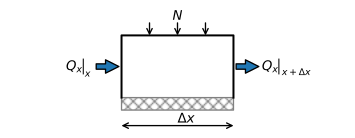
Figure 1.1 Steady water balance in a section of an aquifer that is \(\Delta x\) long and \(\Delta y = 1\) wide in the direction normal to the plane of flow.

      The volume balance is written for a time period \(\Delta t\). Substitution of the appropriate volumes in the volume balance equation ((1.2)) gives

(1.3)\[ \left.Q_x\right|_x\Delta t + N\Delta x \Delta t - \left.Q_x\right|_{x+\Delta x}\Delta t = 0 \]

Division by \(\Delta x\) and \(\Delta t\) and rearrangement of terms gives

(1.4)\[ \frac{\left.Q_x\right|_{x+\Delta x} - \left.Q_x\right|_x}{\Delta x} = N \]

In the limit for \(\Delta x \to 0\) this gives the differential form of the continuity equation for steady one-dimensional horizontal flow

(1.5)\[ \frac{\text{d} Q_x}{\text{d} x} = N \]

The term \(\text{d} Q_x / \text{d} x\) is also known in mathematics as the one-dimensional divergence of the discharge vector. The divergence is the mathematical equivalent of outflow minus inflow of a flow field.

      The transmissivity of an aquifer is approximated as constant in all but the last solution in this chapter. An aquifer with a constant transmissivity may be a confined aquifer with horizontal top and bottom and constant hydraulic conductivity \(k\). Or it can be an unconfined aquifer where the saturated thickness is approximated as constant. Either way, the Dupuit–Forchheimer approximation is adopted so that the head is approximated as constant in the vertical direction. The horizontal flow is distributed equally over the aquifer thickness \(H\) so that the discharge vector \(Q_x\), the integrated specific discharge over the thickness of the aquifer, may be written as

(1.6)\[ Q_x=Hq_x=-T\frac{\text{d}h}{\text{d}x} \]

where \(T=kH\) is the transmissivity of the aquifer and \(q_x\) is given by Darcy’s law (Eq. (9)). The continuity equation for this problem is ((1.5)). Substitution of Eq. ((1.6)) for \(Q_x\) in Eq. ((1.5)) gives

(1.7)\[ \frac{\text{d}}{\text{d}x}\left(T\frac{\text{d}h}{\text{d}x}\right)=-N \]

Because the transmissivity \(T\) is approximated as constant, the differential equation simplifies to

(1.8)\[ \frac{\text{d}^2h}{\text{d}x^2}=-\frac{N}{T} \]

This is a second order, linear, ordinary differential equation known as the Poisson equation. The general solution is obtained by integrating Eq. ((1.8)) twice, which gives, for the case that \(N\) is constant,

(1.9)\[ h=-\frac{N}{2T}x^2 + Ax +B \]

where \(A\) and \(B\) are integration constants that need to be determined from boundary conditions.