9.3. Wells in a semi-confined aquifer

The solution for steady flow to a well in a semi-confined aquifer was presented in Section 6.4. In this section, the equivalent solution is presented for transient flow. Consider a semi-confined aquifer with transmissivity \(T\) and storage coefficient \(S\). The top of the aquifer is formed by a semi-confining layer with resistance \(c\) (Figure 6.12). Storage in the semi-confining layer is neglected. The head \(h^*\) above the semi-confining layer is fixed to zero. Vertical leakage \(q_z\) through the semi-confining layer is computed as Eq. ((2.2))

(9.28)\[ q_z=\frac{h-0}{c} \]

so that the governing differential equation for radial flow is

(9.29)\[ \frac{\partial^2 h}{\partial r^2}+\frac{1}{r}\frac{\partial h}{\partial r}= \frac{S}{T}\frac{\partial h}{\partial t} + \frac{h}{cT} \]

A well starts pumping with discharge \(Q\) at time \(t = t_0\). Initially, the head change caused by the well in the aquifer is equal to zero everywhere. The initial and boundary conditions are the same as those for the Theis solutions ((9.6), (9.7), and (9.8)).
      The solution to this problem was first obtained by Hantush and Jacob (1955) and is referred to as the Hantush function

(9.30)\[ h = -\frac{Q}{4\pi T}\int_u^\infty \frac{1}{\tau}\exp\left(-\tau -\frac{r^2}{4\lambda^2 \tau}\right) \text{d}\tau \]

where \(\lambda=\sqrt{Tc}\) is the leakage factor and \(u\) is defined as for the Theis well

(9.31)\[ u = \frac{S r^2}{4T(t-t_0)} \]

The solution for the case that the head above the semi-confining layer is equal to \(h^*\) rather than zero is obtained by simply adding a constant \(h^*\) to the solution. Note that this is allowed because \(h=h^*\) is a particular solution to the differential equation

(9.32)\[ \frac{\partial^2 h}{\partial r^2}+\frac{1}{r}\frac{\partial h}{\partial r} = S\frac{\partial h}{\partial t} + \frac{h-h^*}{cT} \]

      The seemingly easy integral in the equation for the head (Eq. (9.30)) cannot be integrated analytically, nor is it included in the special functions of the scipy.special package; early literature included tabulated values. The easiest way to compute the integral with Python is to use numerical integration using, e.g., the quad function of the scipy.integrate package. The quad function returns a number of items, of which the first one is the computed integral. In the example code below, the head is first plotted as a function of \(r\) and then plotted as a function of \(t\) (Figure 9.6). The solution for a well in a semi-confined aquifer (Hantush) is compared to the solution for a well in a confined aquifer (Theis). The Hantush and Theis heads are similar for early times when most of the water pumped by the well comes from storage. The Hantush and Theis heads deviate when a significant amount of water pumped by the well comes from leakage through the semi-confining layer. The Hantush solution approaches the steady state solution for a well in a semi-confined aquifer (6.56) in approximately one day for the parameters used in the example below. The Theis solution does not reach steady state, as explained in Section 9.1.

# parameters
T = 200 # transmissivity of aquifer, m^2/d
S = 0.0005 # storage coefficient of aquifer, -
c = 1000 # resistance of leaky layer, d
Q = 800 # discharge of well, m^3/d
rw = 0.3 # radius of well, m
lab = np.sqrt(c * T) # leakage factor, m
print(f'leakage factor: {lab:.2f} m')

leakage factor: 447.21 m

# solution
from scipy.integrate import quad

def integrand(tau, r, T, lab):
    return 1 / tau * np.exp(-tau - r ** 2 / (4 * lab ** 2 * tau))

def hantush(r, t, T, S, c, Q):
    lab = np.sqrt(T * c)
    u = S * r ** 2 / (4 * T * t)
    F = quad(integrand, u, np.inf, args=(r, T, lab))[0]
    return -Q / (4 * np.pi * T) * F

hantushvec = np.vectorize(hantush) # vectorized version of hantush function

# basic plot for one value of r and one value of t
plt.subplot(121)
r = np.linspace(rw, 2 * lab, 100)
t = 6 / 24
plt.plot(r, hantushvec(r, t, T, S, c, Q), label='Hantush')
plt.plot(r, theis(r, t, T, S, Q), label='Theis') # theis func from Section 9.1
plt.legend()
plt.subplot(122)
t = np.linspace(0.01, 2, 100)
r = lab # evaluate head at r=lambda
plt.plot(t, hantushvec(r, t, T, S, c, Q), label='Hantush')
plt.plot(t, theis(r, t, T, S, Q), '--', label='Theis')
plt.legend();

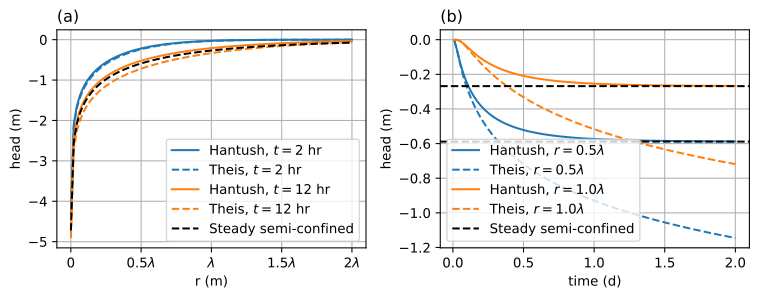
Figure 9.6 Comparison of a well in a semi-confined aquifer (Hantush) vs. a well in a confined aquifer (Theis); head vs. \(r\) (left) and head vs. time (right).

Exercise 9.8

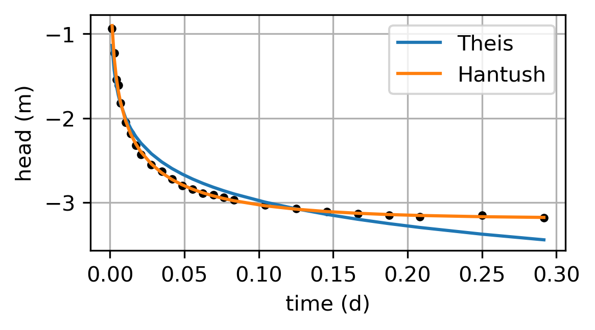
Consider a 7-hour pumping test in a leaky aquifer with discharge \(Q = 24466\) m\(^3\)/d (U.S. Dept. of Interior, Bureau of Reclamation (1995), Texas Hill project, Table 9.5 ). The data in an observation well 24.38 m from the pumping well are given below. First, estimate the transmissivity and storage coefficient approximating the aquifer as confined. Next, estimate the transmissivity, storage coefficient, and resistance of the leaky layer approximating the aquifer as semi-confined. Compute the root-mean squared error, and make a graph of the fit for both models.

Solution

Theis: \(T = 4484\) m\(^2\)/d, \(S = 0.0018\), \(RMSE = 0.12\) m
Hantush: \(T = 3135\) m\(^2\)/d, \(S = 0.0044\), \(c = 25.2\) d, \(RMSE = 0.02\) m

# data Exercise 9.7
t = np.array([2, 4, 6, 8, 10, 15, 20, 25, 30, 40, 50, 60, 70, 80, 90, 100, 
              110, 120, 150, 180, 210, 240, 270, 300, 360, 420]) # minutes
h = np.array([-0.94, -1.23, -1.54, -1.61, -1.82, -2.05, -2.18, -2.32, -2.43,
              -2.55, -2.63, -2.72, -2.8 , -2.84, -2.89, -2.91, -2.94, -2.97,
              -3.03, -3.07, -3.11, -3.13, -3.15, -3.17, -3.15, -3.18]) # m

      As an example, the solution for transient flow to a well that starts pumping at \(t_0 = 0\) in a semi-confined aquifer is repeated here using a Laplace transform solution following the procedure explained in Section 5.4. The same procedure is used to solve the transient flow problems in the next two sections. The Laplace-transform of the differential equation ((9.29)) is

(9.33)\[ \nabla^2 \overline{h} = \frac{Sp}{T}\overline{h} + \frac{\overline{h}}{cT} = w\overline{h} \]

where \(\overline{h}\) is the Laplace-transformed head, \(p\) is the Laplace transform parameter, and

(9.34)\[ w = \frac{Scp + 1}{cT} \]

Boundary conditions ((9.6)) and ((9.8)) transform to

(9.35)\[ \lim_{r \to 0} -2\pi r \overline{Q}_r = \frac{Q}{p} \]

(9.36)\[ \overline{h}|_{r=\infty} = 0 \]

The radial flow problem in the Laplace domain is mathematically analogous to a steady well in a semi-confined aquifer (Section 6.4), and the solution is

(9.37)\[ \overline{h} = -\frac{Q}{2 \pi T p} \text{K}_0\left(r\sqrt{w}\right) \]

Back-transformation to the time domain is conducted numerically using the Stehfest algorithm (see Section 5.4). The example below shows that the Hantush solution using numerical integration of Eq. ((9.30)) is virtually the same as the solution obtained with the Laplace transform technique and the Stehfest algorithm (Figure 9.7).

# Laplace transform solution
def hbar(p, r, T, S, c, Q):
    w = (S * c * p + 1) / (c * T)
    return -Q / (2 * np.pi * T * p) * k0(r * np.sqrt(w))

t = np.linspace(1e-3, 1, 100)
h = stehfest(250, t, hbar, T=T, S=S, c=c, Q=Q) # stehfest func from Section 5.5
h_hantush = hantushvec(250, t, T, S, c, Q)

# basic plot
plt.plot(t, h[0], label='Stehfest')
plt.plot(t, h_hantush, '--', label='Hantush')
plt.legend();

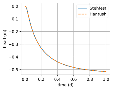
Figure 9.7 Comparison of Laplace transform solution with the numerical integration of the integral in the Hantush solution for a well in a semi-confined aquifer.