4.3. Combined confined/semi-confined interface flow

Section 4.1 and Section 4.2 dealt with interface flow to coastlines that were approximated as vertical. Here, the bottom of the sea is approximated as horizontal and separated from the aquifer by a leaky layer with resistance \(c\) (Figure 4.9). This means that flow in the part of the aquifer below the sea is semi-confined; the thickness of the leaky layer is neglected. As in Section 4.1, flow toward the coast is uniform at a rate \(Q_x=U\), the origin of the coordinate system is chosen at the coast line, and the aquifer extends toward negative infinity. The top and bottom of the aquifer are \(z_t\) and \(z_b\), respectively. Below the land, the aquifer is confined. The length of the outflow zone below the sea is unknown upfront. The sea bottom extends toward positive infinity (or at least beyond the point where the groundwater flow terminates).

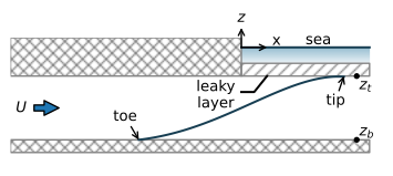
Figure 4.9 Interface flow toward a sea that is separated from the aquifer by a leaky layer.

      The flow problem now consists of three parts: confined flow upstream of the interface toe, confined interface flow between the toe and the coast line, and semi-confined interface flow below the sea. The flow below the land can be solved with the discharge potential for confined interface flow derived in Section 4.1. The discharge potential cannot be used for the semi-confined flow section below the sea.
      An expression for the flow in the semi-confined part is derived below. It is assumed that the toe of the interface is below the land (a condition is derived later). Just as for confined interface flow, the discharge vector below the sea can be written as (see Eq. (4.7))

(4.35)\[ Q_x=-k(\alpha h + z_t)\frac{\text{d}h}{\text{d}x} \]

In the sea, the freshwater head \(h^*\) at elevation \(z_t\) is

(4.36)\[ h^* = -z_t/\alpha \]

so that \(Q_x\) may be written as

(4.37)\[ Q_x = -k\alpha (h-h^*) \frac{\text{d}h}{\text{d}x} \]

The flow below the sea is governed by the differential equation for semi-confined flow

(4.38)\[ \frac{\text{d}Q_x}{\text{d}x} = \frac{h-h^*}{c} \]

Substitution of Eq. ((4.37)) for \(Q_x\) in Eq. ((4.38)) and rearrangement of terms gives

(4.39)\[ \frac{\text{d}^2(h-h^*)^2}{\text{d}x^2}=\frac{2(h-h^*)}{k\alpha c} \]

The boundary conditions are that the discharge vector equals \(U\) at the coastline

(4.40)\[ Q_x\vert_{x=0}=U \]

and that the head equals \(h^*\) at the tip of the interface, which is at the a priori unknown location \(x=x_\text{tip}\)

(4.41)\[ h\vert_{x=x_\text{tip}}=h^* \]

The solution to Eq. ((4.39)) with boundary condition ((4.41)) is

(4.42)\[ h = h^* + \frac{(x-x_\text{tip})^2}{6k\alpha c} {\hskip 2em} 0\le x\le x_\text{tip} \]

It is easy to check this solution by substituting the function and its second derivative in the differential equation ((4.39)) and by evaluating the boundary conditions. An expression for the discharge vector is obtained from differentiation and substitution in Eq. ((4.37)), which gives

(4.43)\[ Q_x=-\frac{(x-x_\text{tip})^3}{18k\alpha c^2} {\hskip 2em} 0\le x\le x_\text{tip} \]

Finally, application of boundary condition ((4.40)) gives

(4.44)\[ x_\text{tip} = (18k\alpha c^2U)^{1/3} \]

Note that this means that the outflow zone has a finite length and depends on the parameters of the aquifer and leaky layer, the density difference, and the total outflow into the sea. This is contrary to regular semi-confined flow (no interface), where the outflow zone is theoretically infinitely long and 95% of the water leaks through the semi-confining layer over a distance of three times the leakage factor (\(\lambda=\sqrt{kHc}\)), independent of the total outflow (Chapter 2).
      The head \(h_0\) at \(x=0\) is obtained from Eq. ((4.42)) as

(4.45)\[ h_0 = h^* + \frac{x_\text{tip}^2}{6k\alpha c} \]

Solution ((4.42)) is only valid if the toe of the interface is not below the sea, which means that

(4.46)\[ h_0<-z_b/\alpha \]

Using that \(z_b=z_t-H=-\alpha h^*-H\) and after some algebra, this gives the following condition for \(U\)

(4.47)\[ U \le \frac{kH^2\sqrt{2/3}}{\alpha \lambda} \]

The solution for the case that the interface toe is below the sea may be found in Bakker (2006).
      Finally, a solution is obtained for the part of the aquifer below the land. The discharge potential at \(x = 0\) is obtained from \(h_0\) (Eq. (4.45)) with the potential for confined interface flow (Eq. (4.8)) as

(4.48)\[ \Phi_0 = \tfrac{1}{2}k\alpha(h_0-h^*)^2 \]

The solution for the discharge potential below the land is

(4.49)\[ \Phi = -U x + \Phi_0 \]

The toe of the interface is located at the point where \(\Phi=\Phi_\text{toe}\) (Eq. (4.9)), which gives

(4.50)\[ x_\text{toe}=-\frac{\Phi_\text{toe}-\Phi_0}{U} \]

In Section 4.1, the coast was approximated as vertical, which is equivalent to the current problem if the resistance of the leaky layer at the bottom of the sea is set to \(c = 0\) in Eq. ((4.45)), which gives \(h_0=h^*\) (note that \(x_\text{tip}\) approaches zero for \(c\to 0\)). In the example below, the same parameters are used as in the example of Section 4.1, and the interface is computed for two values of the resistance of the leaky layer and for \(c\to 0\)(Figure 4.10).

# parameters
k = 10 # hydraulic conductivity, m/d
zt = -10 # top of aquifer, m
zb = -30 # bottom of aquifer, m
alpha = 40 # alpha factor, -
clist = [1e-12, 5, 50] # three values of resistance of leaky layer, d
U = 0.4 # flow towards the coast, m^2/d
H = zt - zb # aquifer thickness, m

# solution
def interface(k, zt, zb, c, alpha, U):
    H = zt - zb
    # below sea
    hstar = -zt / alpha
    xtip = (18 * U * k * alpha * c**2) ** (1 / 3)
    xsea = np.linspace(0, xtip, 100)
    hsea = hstar + (xsea - xtip)**2 / (6 * k * alpha * c)
    h0 = hstar + xtip ** 2 / (6 * k * alpha * c)
    # below land
    phi0 = 0.5 * k * alpha * (h0 - hstar)**2
    phitoe = 0.5 * k * H ** 2 / alpha
    xtoe = -(phitoe - phi0) / U
    Cc = (0.5 * k * H ** 2 + k * H * zb) / alpha
    xland = np.linspace(xtoe, 0, 100)
    phi = -U * xland + phi0
    hland = np.sqrt(2 * phi/ (k * alpha)) + hstar
    # combine solution
    x = np.hstack((xland, xsea))
    zi = -alpha * np.hstack((hland, hsea))
    return x, zi

# basic plot
plt.subplot(111, aspect=4, ylim=(-30, -10))
for c in clist:
    x, zi = interface(k=k, zt=zt, zb=zb, c=c, alpha=alpha, U=U)
    plt.plot(x, zi, label=f'c={c:.0f} d')
plt.legend();

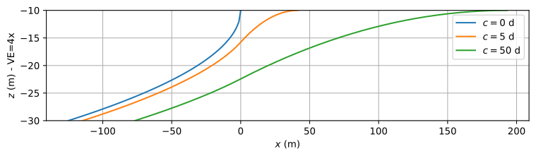
Figure 4.10 Interface elevation for different values of the resistance of the semi-confining layer below the sea.

      The streamlines for the case that \(c = 5\) d are computed below and shown in Figure 4.11.

c = 5
x, zi = interface(k=k, zt=zt, zb=zb, c=5, alpha=alpha, U=U)
x = np.hstack((-200, x))
zi = np.hstack((zb, zi))
Qx = U * np.ones_like(x)
lab = np.sqrt(c * k * H)
xtip = (18 * U * k * alpha * c**2) ** (1 / 3)
Qx[x>0] = -(x[x>0] - xtip) ** 3 / (18 * k * alpha * c**2)
xg = [x, x]
zg = [zi, zt * np.ones_like(x)]
psi = [np.zeros_like(x), Qx]

# basic streamline plot
plt.subplot(111, aspect=2)
plt.contour(xg, zg, psi);

Figure 4.11 Streamlines in a vertical cross section for interface flow toward a sea that is separated from the aquifer by a leaky layer. Discharge between two streamlines is \(\Delta\psi=0.05\) m\(^2\)/d.

Exercise 4.9

Redo the interface flow part of the example presented in Section 4.2, but now the shore line is not vertical, but the sea bottom is horizontal at \(z_t=0\) on both sides of the island and separated from the aquifer by a thin resistance layer with resistance \(c = 5\) d; use \(N = 0.001\) m/d. Compute the head and interface elevation at the shore line (\(x = 0\) or \(x = L\)) and at the center of the island.

Solution

\(h = 0.11\) m, \(z_i = -4.22\) m at shoreline
\(h = 0.404\) m, \(z_i = -16.18\) m at center of island