Flow between a lake and a drained area

2.2. Flow between a lake and a drained area#

One-dimensional flow is modeled between a lake and a drained area, as shown in Figure 2.4. Both the lake and drained area are separated from the aquifer by a semi-confining layer, which has a resistance \(c_0\) below the lake and a resistance \(c_1\) below the drained area. The lake and drained area are separated by a dike of negligible width (the vertical black line at \(x=0\) in the figure). The water level in the lake is \(h_0^∗\), while the water level in the drained area is \(h_1^∗\). The semi-confined aquifer extends to infinity on both sides. The transmissivity of the aquifer is constant and equal to \(T\).

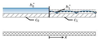
../_images/bccc5fb5c526b4fc105fcacd87e06b6e907e14515fc2126a997f17726a37d9d5.svg — Figure 2.4 Semi-confined flow from a canal to a polder.#

Separate differential equations are written for the part of the aquifer below the lake and the part below the drained area

(2.16)#\[\begin{split} \begin{split} \frac{\text{d}^2(h-h_0^*)}{\text{d}x^2} &= \frac{h-h_0^*}{\lambda_0^2} {\hskip 2em} x\le 0 \\ \frac{\text{d}^2(h-h_1^*)}{\text{d}x^2} &= \frac{h-h_1^*}{\lambda_1^2} {\hskip 2em} x\ge 0 \end{split} \end{split}\]

where \(\lambda_0=\sqrt{c_0T}\) and \(\lambda_1=\sqrt{c_1T}\).
The boundary conditions are that the head approaches \(h_0^*\) far to the left and \(h_1^*\) far to the right

(2.17)#\[ h\vert_{x\to-\infty}=h_0^* {\hskip 2em} h\vert_{x\to+\infty}=h_1^* \]

and continuity requires that the head and flow are continuous across \(x=0\) (see also the conditions at \(x=L_0\) in Section 1.4)

(2.18)#\[ h_{x=0^-}=h_{x=0^+} {\hskip 2em} Q_x|_{x=0^-}=Q_x|_{x=0^+} \]

where the superscripts \(^-\) and \(^+\) stand for evaluation just to the left and just to the right of \(x=0\), respectively.
The solutions for the head below the lake and drained area are written as

(2.19)#\[\begin{split} \begin{split} h=h_0^* + A_0\text{e}^{-x/\lambda_0} + B_0\text{e}^{x/\lambda_0} \hskip 2em x\le 0 \\ h=h_1^* + A_1\text{e}^{-x/\lambda_1} + B_1\text{e}^{x/\lambda_1} \hskip 2em x\ge 0 \\ \end{split} \end{split}\]

Application of the first two boundary conditions gives \(A_0=0\) and \(B_1=0\), after which application of the two continuity conditions gives the following two equations

(2.20)#\[\begin{split} \begin{split} h_0^*+B_0 &= h_1^* + A_1 \\ -T\frac{B_0}{\lambda_0} &= T\frac{A_1}{\lambda_1} \end{split} \end{split}\]

Solving for the two remaining unknowns \(A_1\) and \(B_0\) gives

(2.21)#\[ A_1 = \lambda_1 \gamma \hskip 2em B_0 = -\lambda_0 \gamma \]

where the dimensionless head difference \(\gamma\) is

(2.22)#\[ \gamma = \frac{h_0^* - h_1^*}{\lambda_0 + \lambda_1} \]

The solution for the head now becomes

(2.23)#\[\begin{split} \begin{split} h&=h_0^* -\lambda_0\gamma \text{e}^{x/\lambda_0} \hskip 2em x\le 0 \\ h&=h_1^* + \lambda_1\gamma \text{e}^{-x/\lambda_1} \hskip 2em x\ge 0 \\ \end{split} \end{split}\]

Note that for the case of equal resistance values (so that \(\lambda_0=\lambda_1\)), the head in the aquifer at \(x=0\) is \((h_0^*+h_1^*)/2\) as is to be expected from symmetry when the aquifer properties are the same on both sides of the dike.
The discharge vector is obtained as

(2.24)#\[ Q_x=-T\frac{\text{d}h}{\text{d}x} \]

which gives

(2.25)#\[\begin{split} \begin{split} Q_x&=T\gamma \text{e}^{x/\lambda_0} \hskip 2em x\le 0 \\ Q_x&=T\gamma \text{e}^{-x/\lambda_1} \hskip 2em x\ge 0 \\ \end{split} \end{split}\]

The total flow \(Q_0\) from the lake to the drained area is

(2.26)#\[ Q_0=Q_x|_{x=0}=T\gamma = T \frac{h_0^* - h_1^*}{\lambda_0 + \lambda_1} \]

Note again that 95% of \(Q_0\) has leaked from the lake into the aquifer over a distance of \(3\lambda_0\) to the left of the dike, and 95% of \(Q_0\) has discharged from the aquifer into the drained area over a distance of \(3\lambda_1\) to the right of the dike. In other words, three times the leakage factor away from a disturbance (here, the dike), the head in the aquifer is approximately equal to the head above the semi-confining layer. An example is presented below for the case that \(c_1=4c_0\), so that \(\lambda_1=2\lambda_0\) (Figure 2.5).

# parameters
h0star = 1 # head above left side leaky layer, m
h1star = -1 # head above right side leaky layer, m
k = 10 # hydraulic conductivity, m/d
H = 10 # aquifer thickness, m
c0 = 100 # resistance of left side leaky layer, d
c1 = 400 # resistance of right side leaky layer, d
T = k * H # transmissivity, m2/d
lab0 = np.sqrt(c0 * T) # leakage factor left side, m
lab1 = np.sqrt(c1 * T) # leakage factor right side, m
gamma = (h0star - h1star) / (lab0 + lab1) # dimensionless head difference, -

# solution
x = np.hstack((np.linspace(-5 * lab0, 0, 51), np.linspace(0, 5 * lab1, 51)))
h = np.zeros_like(x)
h[x < 0]  = h0star - lab0 * gamma * np.exp(x[x < 0] / lab0)
h[x >= 0] = h1star + lab1 * gamma * np.exp(-x[x >= 0] / lab1)
Qx = np.zeros_like(x)
Qx[x<0] = T * gamma * np.exp(x[x<0] / lab0)
Qx[x>=0] = T * gamma * np.exp(-x[x>=0] / lab1)
Q0 = T * gamma

# basic plot
plt.subplot(121)
plt.plot(x, h, 'C0')
plt.subplot(122)
plt.plot(x, Qx, 'C1');

../_images/1x1_pixel.png — Figure 2.5 Semi-confined flow between a lake (\(x\le 0\)) and a drained area (\(x\ge 0\)); head (left) and \(Q_x\) (right).#

The stream function is contoured below. There are 20 contour intervals, so that the flow between two adjacent streamlines is 5% of the flow (Figure 2.6). The first streamline that is contoured enters the aquifer at \(x=-3\lambda_0\) and exits at the top of the aquifer at \(x=3\lambda_1\).

# solution
psi = np.zeros((2, len(x)))
psi[1] = -Qx
xg = x
zg = [0, H]

# basic streamline plot
plt.contour(xg, zg, psi, np.linspace(-Q0, 0, 21), colors='C1', linestyles='-');

Exercise 2.3

Consider one-dimensional steady flow into a long and wide lake with a leaky bottom (see Figure 2.7). A coordinate system is chosen such that \(x=0\) at the lake shore. Flow is unconfined for \(x\le 0\) while flow is semi-confined for \(x\ge 0\). Approximate the transmissivity of the aquifer as equal to \(T\) and constant everywhere. The resistance of the leaky semi-confining layer is \(c\), and the water level in the lake is \(h_L\). The discharge vector in the unconfined part of the aquifer is constant and is known from a water balance as \(Q_x=U\). Use \(h_L=0\) m, \(H=10\) m, \(T=20\) m\(^2\)/d, \(U=0.02\) m\(^2\)/d, and \(c=100\) d. Derive and plot an equation for the head as a function of \(x\). In a separate figure, draw streamlines in a vertical cross-section.

Hint

Try the following form of the solution:
\(x \le 0 {\hskip 2em} h=-Ux+h_0\)
\(x \ge 0 {\hskip 2em} h=A\text{e}^{x/\lambda}\)
Solve for \(A\) and \(h_0\) so that the head and flow are continuous at \(x=0\).

Solution

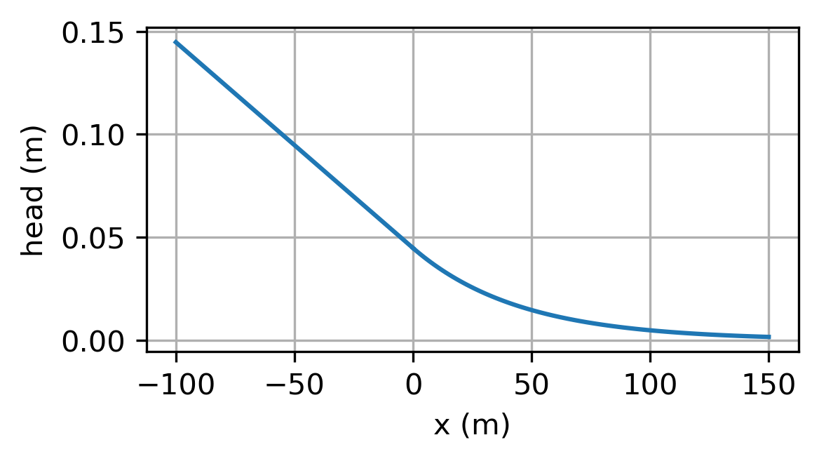
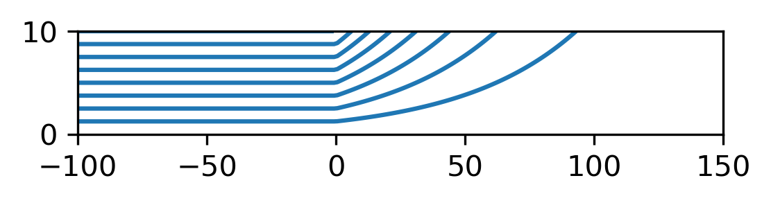
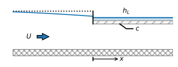
../_images/b5a07e34eea99b200a4e7304d3f9fb272b5edd7f3ff010177fddfdaa8026909a.svg — Figure 2.7 Setup for Exercise 2.3.#