7.4. A well in uniform background flow near the coast

The solutions in the previous section concerned the capture zone of a well in uniform background flow near a straight river. The critical discharge of the well was derived such that the well does not capture water from the river. In this section, the straight river is replaced by a straight and vertical coastal boundary and the maximum discharge of the well is determined such that the well does not pump any salt water. In other words, the maximum discharge is determined such that the interface does not reach the well. It turns out that this maximum discharge is quite a bit smaller than the maximum discharge for a well near a river (Section 7.3).
     Consider a well in a coastal aquifer. The coastline is located along the line \(x=0\). The well is located at \((x,y)=(-d,0)\), has a discharge \(Q\), and a radius \(r_w\). In absence of the well, the flow towards the coast is uniform and equal to \(Q_x=U\). The aquifer is unconfined, the hydraulic conductivity is \(k\) and the elevation of the bottom of the aquifer is \(z_b\) with respect to sea level. The density of the seawater is \(\rho_s\). The sea is in direct contact with the aquifer (no seabed resistance), so that the head along the coastline is equal to sea level. The solution for the discharge potential is identical to the solution for a well near a river in direct contact with the aquifer (see Eq. (7.20)). For this case of unconfined interface flow, the potential at the toe of the interface is (see Eq. (4.26))

(7.27)\[ \Phi_\text{toe} = \tfrac{1}{2}k\frac{\alpha+1}{\alpha^2}z_b^2 \]

In the absence of pumping, the toe of the interface is located at (see Eq. (4.21))

(7.28)\[ x_\text{toe}=-\frac{\Phi_\text{toe}}{U} \]

     First, consider the case that the discharge of the well is half the critical discharge for a well near a river (Eq. (7.24)). A flow net is constructed showing that indeed the stagnation point is still far from the coast line for this value of \(Q\) (Figure 7.7). The toe of the interface in the absence of pumping is plotted with a black dashed line, while the contour line representing \(\Phi_\text{toe}\) for the case with pumping is plotted with a black solid line. It turns out that there are two contour lines where the potential is equal to \(\Phi_\text{toe}\). One contour line runs from North to South and curves towards the well; this is the location of the toe of the interface during pumping. A second black contour is present around the well. This is because the discharge potential at the well is below \(\Phi_\text{toe}\), but this does not mean that the well pumps saltwater. The black contour line around the well is not connected to the black contour line near the coast, which means that there is no way for the saltwater to reach the well. This is further illustrated in the right graph of Figure 7.7, where the potential is plotted as a function of \(x\) along the line \(y=0\). When converting the potential to a head, the values of the potential inside the closed black contour around the well must be converted to a head using the formula for unconfined flow rather than for unconfined interface flow.

# parameters
rw = 0.3 # radius of well, m
k = 40 # hydraulic conductivity, m/d
zb = -20 # elevation of bottom of aquifer, m
rhof = 1000 # density of fresh water, kg/m^3
rhos = 1025 # density of salt water, kg/m^3
U = 1 # uniform flow in x-direction, m^2/d
d = 1000 # dischance of well from coast line, m
Qcr = np.pi * U * d # critical discharge from well near river, m^3/d
Q = Qcr / 2 # discharge of well, m^3/d
print(f'dischage of well: {Q:.2f} m^3/d')

dischage of well: 1570.80 m^3/d

# solution
alpha = rhof / (rhos - rhof) # alpha factor
phitoe = 0.5 * k * (alpha + 1) / alpha ** 2 * zb ** 2
xtoe = -phitoe / U # toe in the absence of pumping

def potential(x, y, Q):
    r1sq = (x + d) ** 2 + y ** 2
    r2sq = (x - d) ** 2 + y ** 2
    return -U * x + Q / (4 * np.pi) * np.log(r1sq / r2sq) 

def streamfunc(x, y, Q, d=d):
    theta1 = np.arctan2(y, x + d)
    theta2 = np.arctan2(y, x - d)
    return -U * y + Q / (2 * np.pi) * (theta1 - theta2)
    
xg, yg = np.meshgrid(np.linspace(-1200, 0, 120), np.linspace(-500, 500, 101))
pot = potential(xg, yg, Q)
psi = streamfunc(xg, yg, Q)

# basic flow net and potential along y=0
plt.subplot(121, aspect=1)
plt.contour(xg, yg, pot, np.arange(-Qcr, Qcr, Qcr / 30), colors='C0')
plt.contour(xg, yg, pot, [phitoe], colors='k')
plt.contour(xg, yg, psi, np.arange(-Qcr, Qcr, Qcr / 30), colors='C1')
plt.axvline(xtoe, color='k', linestyle='--')
plt.subplot(122) # potential along y=0
plt.plot(xg[0], pot[50], label=r'$\Phi(x,0)$')
plt.axhline(phitoe, ls='--', label=r'$\Phi_{toe}$')
plt.legend();

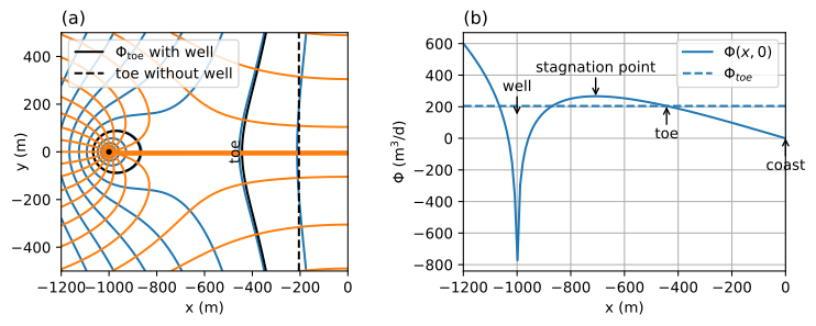
Figure 7.7 A well in uniform background flow towards the coast for a case that \(Q<Q_\text{max}\); flow net (left) and potential along \(y=0\) (right).

     The maximum discharge \(Q_\text{max}\) of the well is reached when the two black contours for \(\Phi_\text{toe}\) touch. This happens when the potential at the stagnation point is equal to \(\Phi_\text{toe}\). The well starts pumping salt water when the discharge is larger than \(Q_\text{max}\) and the presented solution is not valid anymore, as the solution is only valid for stagnant salt water. This is in contrast to the solutions presented in the previous two sections where the solutions were equally valid for well discharges below and above the critical pumping rate \(Q_\text{cr}\).
     The maximum discharge is found numerically. A function is written that takes the discharge \(Q\) as input and returns the difference between the discharge potential at the stagnation point and \(\Phi_\text{toe}\). This function equals zero for the maximum discharge. The brentq method is used to find \(Q_\text{max}\). Note that the maximum discharge is just slightly more than half the critical discharge for a well near a river (Eq. (7.24)).

def func(Q):
    xs = -np.sqrt(d ** 2 - Q * d / (np.pi * U))
    return potential(xs, 0, Q) - phitoe

from scipy.optimize import brentq
Qmax = brentq(func, 1, np.pi * U * d)
print(f'maximum discharge: {Qmax:.2f} m^3/d')
print(f'Qmax as fraction of Qcr of Section 7.3: {Qmax / Qcr:.2f}')
pot1 = potential(xg, yg, Qmax)
psi1 = streamfunc(xg, yg, Qmax)

maximum discharge: 1803.22 m^3/d
Qmax as fraction of Qcr of Section 7.3: 0.57

     When pumping at slightly below the maximum discharge, the toe of the interface is still a significant distance from the well. When the discharge is increased to the maximum discharge, the toe of the saltwater suddenly breaks through to the well as the potential at the stagnation point drops below the potential at the toe; i.e., the head at the stagnation point drops below \(-z_b/\alpha\). An interactive figure is shown below (Figure 7.8); the code is the same as for Figure 7.7 and is not repeated. The potential along the line \(y=0\) shows that the maximum potential between the well and the coast is indeed \(\Phi_\text{toe}\) when \(Q = Q_\text{max}\).

Figure 7.8 A well in uniform background flow towards the coast; flow net (left) and potential along \(y=0\) (right). The red cross is the location of the stagnation point.

Exercise 7.8

The head and interface position for \(Q=Q_\text{max}\) is shown in Figure 7.8. Compute the location of the stagnation point and the head at the well for this case.

Solution

\(h_w=-1.73\) m
\(x_s= -652.7\) m