2. Steady one-dimensional semi-confined flow

In semi-confined aquifers,the aquifer is capped by a leaky layer consisting of a low-permeable material such as peat, shale, or clay. This is in contrast to the confined aquifers considered in the previous chapter, which are capped by a layer that may be approximated as impermeable. The low-permeable layer is referred to as a semi-confining layer or a leaky layer. In what follows, the head above the leaky layer is fixed to a constant level \(h^∗\) (Figure 2.1). This can correspond to the head in an aquifer above the semi-confining layer, or the water level of a surface water body. The fixed head \(h^∗\) can also represent the mean water table in a drained area, where the water table is fixed by means of ditches or tile drains; such drained areas are sometimes referred to as polders. The fixed head \(h^∗\) in the drained area can be in the low-permeable top layer (Figure 2.1) or in a permeable layer separated from the aquifer by a leaky layer (Figure 2.2).

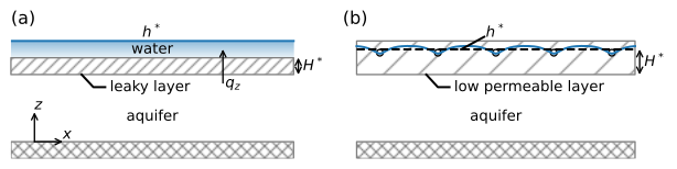
Figure 2.1 Semi-confined aquifer below surface water (left) and semi-confined aquifer below a drained area with a fixed water table in the low permeable layer (right).

      The specific discharge through the leaky layer is approximated as vertical and may be computed with Darcy’s law (Eq. (9)) as

(2.1)\[ q_z = -k^*\frac{\partial h}{\partial z} \approx -k^* \frac{h^*-h}{H^*} \]

where \(h\) is the head in the aquifer, \(h^*\) is the specified head at the top of the leaky layer, \(k^*\) is the vertical hydraulic conductivity of the leaky layer, and \(H^*\) is either the thickness of the leaky layer (left situation of Figure 2.1) or the distance between the drainage level and the bottom of the low permeable layer (right situation of Figure 2.1).
      The specific discharge through the leaky layer is positive for upward flow (in the positive \(z\) direction) and may be written in the form

(2.2)\[ q_z = \frac{h-h^*}{c} \]

where \(c\) [T] is the resistance to vertical flow of the leaky layer defined as

(2.3)\[ c=\frac{H^*}{k^*} \]

Flow in a semi-confined aquifer is governed by the Poisson equation (Eq. (1.8)) where the infiltration rate \(N\) is a function of the head difference across the semi-confining layer. Substitution of \(N=-q_z\) in Eq. ((1.8)) gives

(2.4)\[ \frac{\text{d}^2h}{\text{d}x^2} = \frac{h-h^*}{cT} \]

For the case that \(h^*\) is a constant, this equation can be rewritten as

(2.5)\[ \frac{\text{d}^2(h-h^*)}{\text{d}x^2} = \frac{h-h^*}{\lambda^2} \]

where

(2.6)\[ \lambda=\sqrt{cT} \]

is referred to as the leakage factor [L] and is a characteristic length of the system, as will be explained later.
      Differential equation ((2.5)) is a second-order, linear, ordinary differential equation known as the modified-Helmholtz equation. The general solution is

(2.7)\[ h-h^* = A\text{e}^{-x/\lambda} + B\text{e}^{x/\lambda} \]

where \(A\) and \(B\) are constants to be determined from boundary conditions. The general solution for the discharge vector is

(2.8)\[ Q_x=\frac{AT}{\lambda}\text{e}^{-x/\lambda} - \frac{BT}{\lambda}\text{e}^{x/\lambda} \]

Alternatively, the general solution may be written as

(2.9)\[ h-h^* = A\sinh(x/\lambda) + B\cosh(x/\lambda) \]

with the corresponding discharge vector

(2.10)\[ Q_x=-\frac{AT}{\lambda}\cosh(x/\lambda) - \frac{BT}{\lambda}\sinh(x/\lambda) \]

It depends on the problem whether the formulation in terms of exponential functions or the formulation in terms of hyperbolic functions is more convenient.