5.1. Step changes in surface water level

Changes in river stage propagate as head changes in aquifers that are in contact with the river, which is important for understanding surface water–groundwater interactions. The following example considers one-dimensional transient flow in a semi-infinite aquifer as shown in Figure 5.2. The aquifer is bounded on the left by a fully penetrating river that is in direct contact with the aquifer. Initially, the head in the aquifer is equal to the river stage \(h_l\) everywhere. At time \(t=t_0\), the stage in the river is raised by an amount \(\Delta h\).
     The solution is split into a steady part \(h_s\) that is only a function of \(x\) and a transient part \(h_t\) that is a function of \(x\) and \(t\)

(5.9)\[ h = h_s + h_t \]

The boundary conditions for the steady part are

(5.10)\[ h_s|_{x=0} = h_s|_{x\to\infty} = h_l \]

The steady solution is easy: \(h_s=h_l\).
     The boundary conditions for the transient solution are

(5.11)\[ h_t|_{x=0,t>0} = \Delta h \]

(5.12)\[ h_t|_{x\to\infty, t} = 0 \]

and the initial condition is

(5.13)\[ h_t|_{x, t=0}=0 \]

Note that the sum of the boundary conditions of the steady and transient solutions gives the boundary condition of the stated problem; the same holds for the initial condition. In essence, the transient solution represents the head change in the aquifer caused by the change in the river stage. The remainder of this section is concerned with the transient part of the solution, and the subscript \(_t\) is dropped.

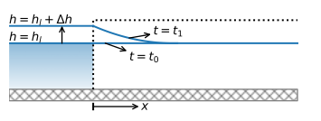
Figure 5.2 Response to an abrupt change in the surface water level (\(t_1>t_0\)).

     The solution to the transient problem was obtained as a similarity solution by Edelman (1947) and is referred to as the Edelman solution. Bruggeman (1999) obtained the same result using the Laplace transform method. The Edelman solution is

(5.14)\[ h(x, t) = \Delta h \, \text{erfc}(u) \]

where

(5.15)\[ u = \sqrt{\frac{Sx^2}{4T(t-t_0)}} \]

and erfc is the complimentary error function defined as

(5.16)\[ \text{erfc}(u) = \int_u^\infty \frac{2}{\sqrt{\pi}} \text{e}^{-\tau^2}\text{d}\tau \]

The complementary error function is available in the scipy.special package.
     An equation for the flux in the aquifer is obtained with Darcy’s law

(5.17)\[ Q_x=-T\frac{\partial h}{\partial x} = -T\Delta h\frac{\partial \text{erfc}(u)}{\partial x} \]

The derivative of the complimentary error function is obtained by first writing

(5.18)\[ \text{erfc}(u) = \int_u^\infty \frac{\text{d} F}{\text{d} \tau} \text{d} \tau = F(\infty) - F(u) \]

where \(F\) is an (unknown) function with derivative

(5.19)\[ \frac{\text{d} F}{\text{d} \tau} = \frac{2}{\sqrt{\pi}} \text{e}^{-\tau^2} \]

The derivative of the complimentary error function may now be written as (note that \(F(\infty)\) does not depend on \(u\))

(5.20)\[ \frac{\partial \text{erfc}(u)}{\partial x} = -\frac{\text{d} F}{\text{d} u} \frac{\partial u}{\partial x} \]

The derivative \(\partial u/\partial x\) is obtained by application of the chain rule

(5.21)\[ \frac{\partial u}{\partial x} = \frac{1}{2}\left( \frac{Sx^2}{4T(t-t_0)} \right)^{-1/2} \frac{2Sx}{4T(t-t_0)} = \frac{1}{u}\frac{u^2}{x}=\frac{u}{x} \]

so that finally

(5.22)\[ Q_x= T\Delta h \frac{2u}{x\sqrt{\pi}} \text{e}^{-u^2} \]

     In the example below, the head and discharge vector are plotted as a function of \(x\) for three different times (Figure 5.3). The variation of the head with \(x\) shows where the additional water is stored in the aquifer. The amount of water that flows from the river into the aquifer decreases quickly, as can also be seen from the graph of \(Q_x\). At \(t=1\) d, the inflow at \(x=0\) is more than 5 m\(^2\)/d and decreases to almost zero at \(x=100\) m. At \(t=100\) d, the inflow at \(x=0\) has decreased to around 0.5 m\(^2\)/d and is still around 0.5 m\(^2\)/d at \(x=200\) m, which means that most water is carried beyond this point to increase storage in the aquifer.

# parameters
T = 100 # transmissivity, m^2/d
S = 0.2 # storage coefficient, -
delh = 2 # change in river level, m
t0 = 0 # time of change in river level, d

# solution
from scipy.special import erfc

def h_edelman(x, t, T, S, delh=1, t0=0):
    u = np.sqrt(S * x ** 2 / (4 * T * (t - t0)))
    return delh * erfc(u)

def Qx_edelman(x, t, T, S, delh, t0=0):
    u = np.sqrt(S * x ** 2 / (4 * T * (t - t0)))
    return T * delh * 2 * u / (x * np.sqrt(np.pi)) * np.exp(-u ** 2) 

# basic plot head and Qx vs x
x = np.linspace(1e-12, 200, 100)
plt.subplot(121)
for t in [1, 10, 100]:
    h = h_edelman(x, t, T, S, delh, t0)
    plt.plot(x, h, label=f'time={t} d')
plt.legend()
plt.subplot(122)
for t in [1, 10, 100]:
    Qx = Qx_edelman(x, t, T, S, delh, t0)
    plt.plot(x, Qx, label=f'time={t} d');

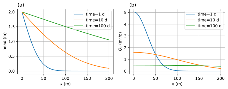
Figure 5.3 Snapshots of the groundwater level in response to an abrupt change in the surface water level; head (left) and \(Q_x\) (right).

     In the following graphs, the head and \(Q_x\) are plotted as a function of \(t\) at three different distances from the river (Figure 5.4). The head as a function of \(t\) represents the head in an observation well. Note that the farther away an observation well is from the river, the longer it takes before the head starts to rise after the river stage is changed. The discharge vector \(Q_x\) shows a clear maximum near the river, but the peak becomes less pronounced as the distance to the river increases.

# basic plot head and Qx vs t
t = np.linspace(1e-12, 100, 100)
plt.subplot(121)
for x in [50, 100, 200]:
    h = h_edelman(x, t, T, S, delh, t0)
    plt.plot(t, h, label=f'distance {x} m')
plt.legend()
plt.subplot(122)
for x in [50, 100, 200]:
    Qx = Qx_edelman(x, t, T, S, delh, t0)
    plt.plot(t, Qx, label=f'distance {x} m')
plt.legend();

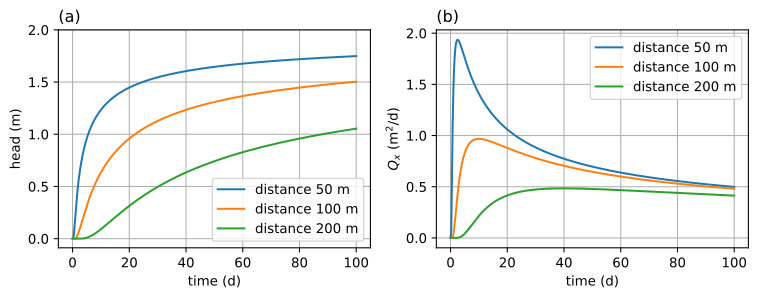
Figure 5.4 Groundwater response in an observation well due to an abrupt change in the surface water level at \(t=0\); head (left) and \(Q_x\) (right).

     According to the solution, it takes infinite time before the head is raised by \(\Delta h\) everywhere in the aquifer. The head far away can only be raised if water flows from the river into the aquifer, which means that the head in the aquifer must be lower than the head in the river everywhere. This means that the gradient from the river to the point where the head is still near the initial head becomes smaller and smaller, so raising the head will go slower and slower. This is an artifact of the approximation that the aquifer extends to infinity, while in reality, some boundary will be present.
     The solution for the head (Eq. (5.14)) is only a function of the dimensionless parameter \(u\), also referred to as the similarity variable (which combines the independent variables). That means that for one specific value of \(u\), there is only one value for the head. For example, the head change at \(x=100\) m and \(t=10\) d may be computed as

x = 100 # m
t = 10 # d
T = 100 # m^2/d
S = 0.2 # -
print(f'head at x = {x} m, t = {t} d for T = {T} and S = {S}:')
print(f'u = {np.sqrt(S * x ** 2 / (4 * T * t)):.3f}')
print(f'h = {h_edelman(x, t, T, S, delh):.6f} m')

head at x = 100 m, t = 10 d for T = 100 and S = 0.2:
u = 0.707
h = 0.634621 m

     If the storage coefficient is not \(S=0.2\) but \(S=0.002\), the same head change at \(x=100\) m is reached after 0.1 d, because \(S=0.002\) and \(t=0.1\) d give the same value of \(u\).

t = 0.1 # d
S = 0.002 # -
print(f'head at x = {x} m, t = {t} d for T = {T} and S = {S}:')
print(f'u = {np.sqrt(S * x ** 2 / (4 * T * t)):.3f}')
print(f'h = {h_edelman(x, t, T, S, delh):.6f} m')

head at x = 100 m, t = 0.1 d for T = 100 and S = 0.002:
u = 0.707
h = 0.634621 m

Exercise 5.1

Consider the case when \(T = 100\) m\(^2\)/d, \(S = 0.2\), \(\Delta h=2\) m. The head at \(x=100\) m and \(t=10\) d is \(h=0.635\) m. For what value of the transmissivity is the head at \(x=100\) m and \(t=10\) d the same when \(S=0.002\) rather than \(S=0.2\)?

Solution

\(T=1\) m\(^2\)/d

Exercise 5.2

Consider the case when \(T = 100\) m\(^2\)/d, \(S = 0.2\), \(\Delta h=2\) m. The head at \(x=100\) m and \(t=10\) d is \(h=0.635\) m. At what distance from the river is the head change at \(t=10\) d the same when \(S=0.002\)?

Solution

\(x=1000\) m

     The accuracy and correct implementation of the solution can be verified in three ways. First, it can be verified that the mathematical solution ((5.14)) is indeed the solution to the stated mathematical problem by checking that the solution satisfies the boundary and initial conditions (Eqs. (5.11)-(5.13)), and by taking derivatives of the solution and substituting them in the governing differential equation ((5.8)) to check that the solution satisfies the differential equation. Second, the Python implementation of the solution may be verified by checking that the solution meets the differential equation and the boundary and initial conditions using accurate numerical derivatives (this approach was applied in Section 2.1).

Exercise 5.3

Verify that solution ((5.14)) meets the differential equation and the boundary and initial conditions, and verify that \(Q_x=-T\text{d}h/\text{d}x\). Use accurate numerical derivatives (see, e.g., Section 2.1).

Solution

Use Eq. (2.14) and Eq. (2.15).

     The third approach to verify the solution is to check the water balance. The total inflow into the aquifer over a period \(\Delta t\) can be computed and compared to the increase in the storage of water in the aquifer. The total inflow can be computed through integration of \(Q_x\) at \(x=0\). \(Q_x\) at \(x=0\) may be obtained from ((5.22)) and ((5.15)) as

(5.23)\[ Q_x|_{x=0,t} = \Delta h \sqrt{\frac{ST}{\pi (t-t_0)}} \]

The total inflow over a period \(\Delta t\) is

(5.24)\[ Q_{in} = \int_{t_0}^{t_0+\Delta t} Q_x|_{x=0,t} = 2 \Delta h \sqrt{\frac{ST \Delta t}{\pi}} \]

The total increase in the storage may be computed through numerical integration along \(x\) of the head in the aquifer at \(t=\Delta t\) and multiplication by the storage coefficient. The integration may be carried out, for example, by using the quad method of scipy.integrate. The total increase in storage must equal the total inflow, as is verified below.

delt = 10 # time period for which water balance is checked
Qin = 2 * delh * np.sqrt(S * T * delt / (np.pi))
from scipy.integrate import quad
stored = S * quad(h_edelman, 1e-12, np.inf, args=(delt, T, S, delh, 0))[0]
print(f'total inflow from river  : {Qin:.6f} m^3')
print(f'total increase in storage: {stored:.6f} m^3')

total inflow from river  : 3.191538 m^3
total increase in storage: 3.191538 m^3

     As the governing differential equation ((5.8)) is linear, solutions may be superimposed through time. For example, if the water level in the river is raised by \(\Delta h_0\) at time \(t_0\) and then again by another \(\Delta h_1\) at time \(t_1\) (where \(t_1>t_0\)), then the transient solution is

(5.25)\[ h(x, t) = \Delta h_0 \text{erfc}(u_0) {\hskip 2em} t_0\le t \le t_1 \]

(5.26)\[ h(x, t) = \Delta h_0 \text{erfc}(u_0) + \Delta h_1 \text{erfc}(u_1) {\hskip 2em} t \ge t_1 \]

where

(5.27)\[ u_0 = \sqrt{\frac{Sx^2}{4T(t-t_0)}} {\hskip 2em} u_1 = \sqrt{\frac{Sx^2}{4T(t-t_1)}} \]

     Consider the following sequence of four steps delh in the river level starting at four different times t0.

delh = np.array([1, 1, -2, 1]) # sequence of river stage changes, m
t0 = np.array([0, 10, 20, 30]) # sequence of times of changes, d

     The transient solution is obtained through superposition of four changes in the river level. A loop is used to compute and plot the head vs. time at 10 and 100 m from the river (Figure 5.5). The solution is presented as an animation.

# solution
t = np.linspace(1e-3, 40, 400) # start jus after t=0
h10 = np.zeros(len(t))
h100 = np.zeros(len(t))
for i in range(len(t0)):
    h10[t > t0[i]] += h_edelman(10, t[t > t0[i]], T, S, delh[i], t0[i])
    h100[t > t0[i]] += h_edelman(100, t[t > t0[i]], T, S, delh[i], t0[i])

# basic plot head (bottom graph)
plt.plot(t, h10, label='x=10 m')
plt.plot(t, h100, label='x=100 m')
plt.legend();

Once Loop Reflect

Figure 5.5 Head response due to a varying surface water level.

     An interesting practical application is the analysis of the passage of a flood wave in the river. The river stage is raised by \(\Delta h\) for a period of \(\Delta t\), after which the level goes back to the initial level. The head rise in the aquifer is obtained from superposition as

(5.28)\[ h(x, t) = \Delta h[\text{erfc}(u_0) - \text{erfc}(u_1)] {\hskip 2em} t \ge \Delta t \]

where

(5.29)\[ u_0 = \sqrt{\frac{Sx^2}{4Tt}} {\hskip 2em} u_1 = \sqrt{\frac{Sx^2}{4T(t-\Delta t)}} \]

The analysis of the groundwater response to a flood wave to estimate aquifer properties is sometimes referred to as the flood wave method. In this case, solution (5.28) may be fitted to estimate the aquifer diffusivity.
     The groundwater response to a flood wave declines with the distance from the river. The distance from the river where the response is negligible (for example, a fraction of \(\Delta h\)) may be computed from solution ((5.28)), but that requires a numerical rootfinding procedure. In practice, the distance where the maximum head response is a fraction \(\alpha\) of the height of the flood wave may be estimated with

(5.30)\[ x \approx \sqrt{\frac{T\Delta t}{S\alpha}} \]

For example, a maximum response of \(0.01\Delta h\) (\(\alpha=0.01\)) is reached at \(x\approx 10\sqrt{T\Delta t/S}\). The time at which the maximum occurs is

(5.31)\[ t_\text{peak} =\frac{Sx^2}{6T} \]

The assessment of the accuracy of the approximate formula ((5.30)) is part of the exercises below.

Exercise 5.4

Consider a flood wave that passes through the river with \(\Delta h=2\) m and \(\Delta t=10\) d. Other parameters are as in the example. Use the approximate formula ((5.30)) to estimate the location where the head response is \(0.01\Delta h\). At this location, plot the head variation vs. time. Make sure that time varies from 0 to \(5t_\text{peak}\). Assess whether the approximate formula works reasonably well by computing the actual maximum head at the location computed with the approximate formula.

Solution

Actual maximum head: 0.0185 m

Exercise 5.5

For the flood wave of the previous exercise, compute and plot the total amount of water stored in the aquifer (on one side of the river) vs. time, for time going from 0 to \(10\Delta t\). How much water is stored in the river bank at \(t=\Delta t=10\) d? And how much at \(t=4\Delta t=40\) d?

Solution

\(V=31.9\) m\(^3\)/m after 10 days
\(V=8.6\) m\(^3\)/m after 40 days