10.2. Flow to a partially penetrating stream

A typical approximation in the development of analytical solutions is that a stream fully cuts through the aquifer. Most streams, however, penetrate only part of the aquifer. Such streams are called partially penetrating streams. In this section, the flowfield around a narrow partially penetrating stream is investigated. A solution is presented for two-dimensional flow in the vertical plane and compared to the Dupuit solution.
      The flow system consists of a confined aquifer with hydraulic conductivity \(k\) and thickness \(H\), and is penetrated by a narrow stream over a distance \(d\) (Figure 10.2). The water level in the stream equals \(h_s\). The width of the stream is approximated as negligible (even though it has a small width in the figure). Flow near infinity on the left equals \(Q_x = U_l\) while flow near infinity on the right equals \(Q_x=U_r\).

(10.17)\[ \lim_{x\to -\infty}Q_x = U_l \]

(10.18)\[ \lim_{x\to \infty}Q_x = U_r \]

(10.19)\[ h|_{x=0,-d\le z\le 0}=h_s \]

      The solution to the stated problem is obtained with conformal mapping. A conformal mapping is a coordinate transformation (a change of variables) for which the Laplace equation is invariant. Some boundary conditions, including a specified head boundary and an impermeable boundary, are also invariant to a conformal transformation. The utility of a conformal mapping is to simplify the problem domain without altering the differential equation or boundary conditions. An analytic solution is then obtained in the simplified domain. The problem domain is also referred to as the physical plane and the simplified transformed domain is called the reference plane.
      A conformal mapping solution is often written in parametric form as \(\omega(\tau)\) and \(\zeta(\tau)\), where \(\tau\) is a reference plane. Here, the reference plane \(\tau=\xi + i\eta\) is chosen as the quarter plane \(\xi\ge 0\) and \(\eta \ge 0\), as shown in Figure 10.2 (note that \(\xi\) (xi) and \(\zeta\) (zeta) look similar but \(\xi\) has a double squiggle and \(\zeta\) just a single squiggle). The top and bottom of the aquifer correspond to the positive real axis of \(\tau\) (note the corresponding green, red, and purple sections in the \(\zeta\) and \(\tau\) planes), while the partially penetrating stream corresponds to the positive imaginary axis in the \(\tau\) plane (the blue section).
      One of the characteristics of a conformal mapping is that there are three degrees of freedom to make a mapping unique; the locations of three boundary points can be chosen in the reference plane. Here it is chosen that point 1 corresponds to \(\tau=1\), point 2 corresponds to \(\tau=\infty\), and point 4 corresponds to \(\tau=0\). Point 3 is located on the imaginary axis in the \(\tau\) plane and point 5 is located between \(\tau=0\) and \(\tau=1\) on the real axis in the \(\tau\) plane, but their exact location is determined by the mapping.

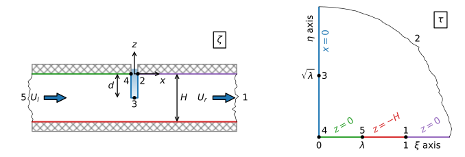
Figure 10.2 Flow to a partially penetrating stream; physical \(\zeta\) plane (left) and the reference \(\tau\) plane (right) with the boundary conditions for \(\zeta=x+iz\).

      The solution for \(\zeta\) as a function of \(\tau\), referred to in conformal mapping jargon as the map of \(\tau\) onto \(\zeta\), is

(10.20)\[ \zeta = x + iz = -\frac{H}{\pi}\ln\left(\frac{\tau - 1}{\tau + 1}\right) + \frac{H}{\pi}\ln\left(\frac{\tau - \lambda}{\tau + \lambda}\right) \]

where

(10.21)\[ \lambda = \left(-\mu + \sqrt{\mu^2 + 1}\right)^2 \]

and

(10.22)\[ \mu = \tan\left(\frac{\pi d}{2H}\right) \]

The parameters \(\mu\) and \(\lambda\) depend on the geometry of the problem (i.e., the relative depth of penetration of the stream \(d/H\)) and not on the flow. For this case, it is possible to invert \(\zeta(\tau)\) to obtain \(\tau(\zeta)\)

(10.23)\[ \tau = -\frac{(Z+1)(\lambda-1)}{2(Z-1)} + \frac{1}{2}\sqrt{\left(\frac{(Z+1)(\lambda - 1)}{Z-1}\right)^2 + 4\lambda} \]

where

(10.24)\[ Z = \text{e}^{\pi\zeta / H} \]

It can be checked analytically that Eq. ((10.20)) fulfills all the boundary conditions. Note that the solution for \(\zeta\) consists of two log terms. Each log term is mathematically equivalent to a well and its image across the imaginary axis in the reference plane (compare Section 6.2). As such the real part of \(\zeta\) (\(x\)) is constant along the imaginary axis in the \(\tau\) plane and the imaginary part is piecewise constant along the real axis in the \(\tau\) plane. It can also be verified numerically that all boundary conditions are met and the solution is implemented correctly in Python by evaluation of \(\zeta\) at points along the boundary in the \(\tau\) plane. An example for a point between points 1 and 2 in the \(\tau\) is shown below. The section between points 1 and 2 corresponds to \(z=0\) and \(x\ge 0\) (see Figure 10.2).

# parameters
k = 10 # hydraulic conductivity, m/d
H = 10 # thickness of aquifer, m
d = 4 # depth of stream, m
Ul = 0.2 # uniform flow far to the left, m^2/d
Ur = -0.2 # uniform flow far to the right, m^2/d
hs = 0 # water level in stream

# solution
def zetafunc(tau, H=H, d=d):
    mu = np.tan(np.pi * d / (2 * H))
    lab = (-mu + np.sqrt(mu**2 + 1))**2
    z = -H / np.pi * np.log((tau - 1) / (tau + 1)) + \
         H / np.pi * np.log((tau - lab) / (tau + lab))
    return z

def taufunc(zeta, H=H, d=d):
    mu = np.tan(np.pi * d / (2 * H))
    lab = (-mu + np.sqrt(mu**2 + 1))**2
    Z = np.exp(np.pi * zeta / H)
    tau = (1 - lab) * (Z + 1) / (2 * (Z - 1)) + 0.5 * np.sqrt(
          ((lab - 1) * (Z + 1) / (Z - 1)) ** 2 + 4 * lab)
    return tau

# verification 
tau = 1.5 + 0j
zeta = zetafunc(tau)
print(f'given tau between points 1 and 2: {tau:.2f}')
print(f'zeta between points 1 and 2: {zeta:.2f}')
print(f'tau as function of zeta: {taufunc(zeta):.2f}')

given tau between points 1 and 2: 1.50+0.00j
zeta between points 1 and 2: 4.01+0.00j
tau as function of zeta: 1.50+0.00j

      The solution for the complex potential is obtained next. The stream function is chosen to equal \(\psi=0\) along the top of the aquifer to the right of the stream (the purple section between points 1 and 2), so that \(\psi=U_r\) along the bottom of the aquifer (the red section between points 5 and 1), and \(\psi=U_r-U_l\) along the top of the aquifer to the left of the stream (the green section between points 5 and 4). The boundary conditions for \(\omega\) in the reference plane \(\tau\) are shown in the left graph of Figure 10.3.
      The solution for \(\omega(\tau)\) in the reference plane may, for this case, be constructed directly in the reference plane with the method of images. Point 5, which is at infinity to the left in the \(\zeta\) plane corresponds to the point \(\xi=\lambda\) in the \(\tau\) plane. There is an amount \(U_l\) flowing from infinity towards the partially penetrating stream. Hence, the solution for \(\omega\) needs an injection well with injection rate \(2U_l\) at point 5. The factor of 2 is needed as only half the water that is injected flows into the upper half plane (\(z\ge 0\)), while the other half flows into the lower half plane (\(z\le 0\)). Similarly, point 1, which is at infinity to the right in the \(\zeta\) plane, corresponds to the point \(\xi=1\) in the \(\tau\) plane. An amount \(U_r\) is taken out at point 1, which means that a well with discharge \(2U_r\) is placed at point 1. Image wells are used to make sure that the potential is equal to \(\phi_s=kh_s\) along the imaginary axis (corresponding to the stream), so that the function for \(\omega\) becomes

(10.25)\[ \omega = \phi + i\psi = -\frac{U_l}{\pi}\ln\left(\frac{\tau - \lambda}{\tau + \lambda}\right) + \frac{U_r}{\pi}\ln\left(\frac{\tau - 1}{\tau + 1}\right) + \phi_s \]

The potential may be evaluated at a point (\(\zeta\)) by first computing \(\tau\) for the specified value of \(\zeta\) with Eq. ((10.23)), followed by evaluation of \(\omega\) with Eq. ((10.25)).
      An example is presented for the case that the flow is the same from both sides of the stream. A flow net in the \(\tau\)-plane is shown in the right graph of Figure 10.3. A flow net in the problem domain is shown in Figure 10.4 . For a fully penetrating stream, the head contours \(h=0.02\) and \(h=0.04\) m are 10 and 20 m from the stream, respectively (these contours are shown in black in Figure 10.4). Note that the vertical head variation is negligible at approximately one aquifer thickness from the partially penetrating stream.

# solution
def omegafunc(tau, Ul=Ul, Ur=Ur, H=H, d=d, k=k, hs=0):
    mu = np.tan(np.pi * d / (2 * H))
    lab = (-mu + np.sqrt(mu**2 + 1))**2
    om = -Ul / np.pi * np.log((tau - lab) / (tau + lab)) + \
          Ur / np.pi * np.log((tau - 1) / (tau + 1)) + k * hs
    return om

# omega transformed domain
xi, eta = np.meshgrid(np.linspace(0, 2, 100), np.linspace(0, 1.5, 100))
om_ref_plane = omegafunc(xi + eta * 1j)
# omega physical domain
xg, zg = np.meshgrid(np.linspace(-4 * H, 4 * H, 400), np.linspace(-H, 0, 100))
taug = taufunc(xg + zg * 1j)
omega = omegafunc(taug)
h = omega.real / k

# basic flow net
plt.subplot(111, aspect=1, xlim=(-40, 10))
plt.contour(xg, zg, h, np.arange(0, 0.1, 0.0025), colors='C0')
plt.contour(xg, zg, omega.imag, np.arange(-0.4, 0.4, 0.025), colors='C1');

# basic plot flow net in transformed domain (right graph)
plt.subplot(111, aspect=1)
plt.contour(xi, eta, om_ref_plane.real, 20, colors='C0')
plt.contour(xi, eta, om_ref_plane.imag, 20, colors='C1')

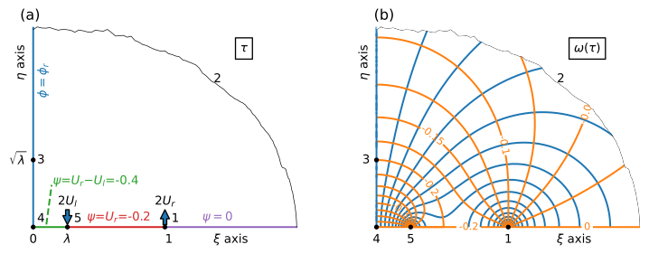
Figure 10.3 Boundary conditions for \(\omega\) in the reference plane (left) and flow net in the reference plane (right).

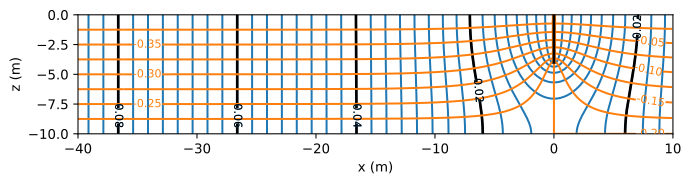
Figure 10.4 A flow net for flow to a partially penetrating stream in an isotropic aquifer.

      The solution for an anisotropic hydraulic conductivity is obtained through application of the procedure outlined in the previous section. The flow net is quite different for the case that the vertical hydraulic conductivity is ten times smaller than the horizontal hydraulic conductivity, as shown in Figure 10.5. The vertical head variation is negligible at ~\(3H\approx H\sqrt{k_x/k_z}\) from the stream.

# anisotropic parameters
kx = 10 # m/d
kz = 1 # m/d

# anisotropic solution
ktilde = np.sqrt(kx * kz)
xgtilde = xg * np.sqrt(kz / kx)
zgtilde = zg
omega_aniso = omegafunc(taufunc(xgtilde + zgtilde * 1j))
h_aniso = omega_aniso.real / ktilde
psi_aniso = omega_aniso.imag

# basic flow net
plt.subplot(111, aspect=1, xlim=(-40, 10))
plt.contour(xg, zg, h_aniso, np.arange(0, 0.2, 0.002), colors='C0')
plt.contour(xg, zg, psi_aniso, np.arange(-0.4, 0.4, 0.02), colors='C1');

Figure 10.5 A flow net for flow to a partially penetrating stream in an anisotropic aquifer.

      The presented solution is compared to the Dupuit solution for one-dimensional flow towards a stream. First, the Dupuit solution is presented for the case that the head in the aquifer at the stream, \(h_0\), is equal to the head in the stream, \(h_s\), over the entire aquifer thickness

(10.26)\[ h_0=h_s \]

The boundary conditions to the left and right are Eqs. ((10.17)) and ((10.18)), respectively. The Dupuit solution is

(10.27)\[\begin{split} \begin{split} h &= -U_lx/T + h_0 {\hskip 2em} x\le 0 \\ h &= -U_rx/T + h_0 {\hskip 2em} x\ge 0 \end{split} \end{split}\]

The Dupuit solution is compared to the two-dimensional solution for the example with anisotropic hydraulic conductivity in Figure 10.6. Note that away form the stream the difference between the Dupuit solution and the head at the top and bottom of the aquifer becomes constant.

# Dupuit solution
L = 40 # distance over which Dupuit solution is computed
h0 = 0
xdupuit = [-L, 0, L]
hdupuit1 = [Ul * L / (k * H) + h0, h0, -Ur * L / (k * H) + h0]

# basic plot
plt.plot(xg[0], h_aniso[-1], 'C0', label='$z=0$')
plt.plot(xg[0], h_aniso[0], 'C0--', label='$z=-H$')
plt.plot(xdupuit, hdupuit1, 'C3', label='Dupuit w/o $C$')
plt.legend(loc='lower right');

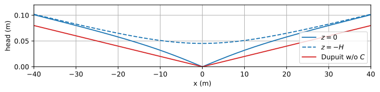
Figure 10.6 Head vs. \(x\) at the top and bottom of an anisotropic aquifer with \(k_z=k_x/10\) compared to the Dupuit solution with \(h\big|_{x=0}=0\).

      Streamlines converge when water approaches the partially penetrating stream, which results in additional head loss that is not taken into account in the Dupuit solution. The additional head loss can be taken into account in the Dupuit solution by replacing the boundary condition at the stream by

(10.28)\[ U_l - U_r = C(h_0 - h_s) \]

where \(U_l-U_r\) is the outflow into the stream, and \(C\) is the effective conductance. The effective conductance \(C\) is computed as

(10.29)\[ C = (U_l - U_r) / (\overline{h}_0 - h_s) \]

where \(\overline{h}_0\) is the average head in the aquifer at \(x=0\) and is obtained from numerical integration of the two-dimensional solution. The effective conductance is a function of the geometry of the problem (\(H\) and \(d\)) and the hydraulic conductivity (\(k_x\) and \(k_z\)), but not of the flow towards the stream (\(U_r - U_l\)). Once \(C\) is known, the head \(h_0\) at \(x=0\) in the Dupuit solution can be computed for any combination of \(U_r\) and \(U_l\) as

(10.30)\[ h_0 = h_s + (U_l - U_r) / C \]

      In the code cell below, the effective conductance \(C\) is computed from the average head \(\overline{h}_0\) for the anisotropic example presented above. The Dupuit solution with the effective conductance is shown in Figure 10.7 and indeed matches the head in the aquifer at a distance of ~\(3H\) from the stream.

# computation of C
def head0(z, Ul=Ul, Ur=Ur, H=H, d=d):
    zeta = 0 + z * 1j
    tau = taufunc(zeta, H=H, d=d)
    return omegafunc(tau, Ul=Ul, Ur=Ur, H=H, d=d).real / np.sqrt(kx * kz)

from scipy.integrate import quad
h0avg = quad(head0, a=-H, b=0, args=(Ul, Ur))[0] / H
C = (Ul - Ur) / (h0avg - 0)
print(f'Effective conducatance: C={C:.2f} m^2/d')
print(f'Dupuit head h0={h0avg:.3f} m for Ul={Ul} m^2/d and Ur={Ur} m^2/d')

Effective conducatance: C=18.70 m^2/d
Dupuit head h0=0.021 m for Ul=0.2 m^2/d and Ur=-0.2 m^2/d

# Dupuit solution with effective conductance
h0 = hs + (Ul - Ur) / C
hdupuit2 = [Ul * L / (k * H) + h0, h0, -Ur * L / (k * H) + h0]

# basic plot
plt.plot(xg[0], h_aniso[-1], 'C0', label='$z=0$')
plt.plot(xg[0], h_aniso[0], 'C0--', label='$z=-H$')
plt.plot(xdupuit, hdupuit2, 'C3', label='Dupuit w/ $C$')
plt.legend(loc='lower right');

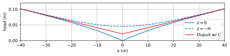
Figure 10.7 Head vs. \(x\) at the top and bottom of an anisotropic aquifer with \(k_z=k_x/10\) compared to the Dupuit solution with effective conductance \(C\).

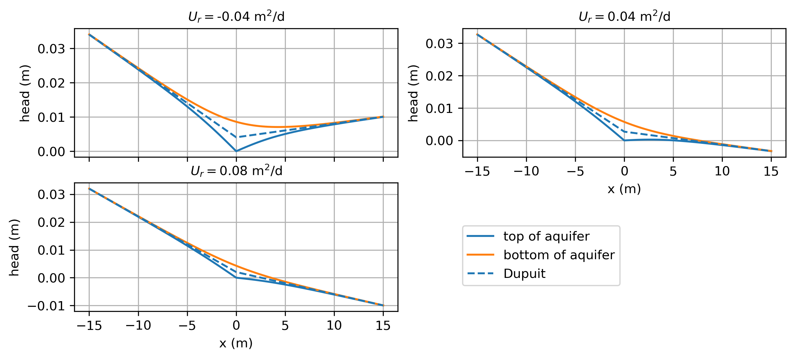
      The flow field gets more interesting when the inflow from the left is not equal to the inflow from the right (\(U_l\ne -U_r\)). Three cases are distinguished here; the flow \(U_l\) from the left is positive for all three cases. For case 1, water flows to the stream from both sides (\(U_r<0\)), which results in a stagnation point along the base of the aquifer. For case 2, the flow on the right side is away from the stream but not too large (\(0 \le U_r \le \lambda U_l\)). As a result, only part of the water that flows to the stream from the left is captured by the stream and the remainder flows under the stream to the right. There is a stagnation point along the top of the aquifer, and water flows into the stream over the entire stream boundary. For case 3, flow on the right side is away from the stream and larger (\(U_r \ge \lambda U_l\)). For this case, water flows into the stream over part of the stream boundary and out of the stream along the other part. The code for the flow nets is the same as for Figure 10.4 and is not repeated. The different cases may be simulated by adjusting the slider in Figure 10.8.

Figure 10.8 Flow nets for different values of \(U_r\). For this case, \(\lambda U_l = 0.052\) m\(^2\)/d so that (part of) the stream starts losing water on the right side when \(Q_r>0.052\) m\(^2\)/d.

Exercise 10.1

Plot the head as a function of \(x\) at the top and bottom of the aquifer (like Figure 10.6) for three cases: \(U_r=-0.04\), \(0.04\), and \(0.08\) m\(^2\)/d; also add the Dupuit solution with effective conductance \(C\).

Solution

Effective conductance (same for all cases): \(C=59.12\) m\(^2\)/d