2.5. Areal recharge between two rivers in a two-aquifer system

The solution for flow between two rivers with areal recharge \(N\) in a single aquifer (Section 1.2) is expanded to two aquifers, where the rivers cut through the top aquifer, but not the bottom aquifer (see Figure 2.14). The two-aquifer solution is used to investigate when the leaky layer and the aquifer below it have a significant effect on the head in the top aquifer or when the bottom of the top aquifer may be approximated as impermeable. The origin is chosen halfway between the two rivers and the distance between the two rivers is \(2L\). The heads in the two rivers are equal to \(h_R\) so that the boundary conditions in the top aquifer are

(2.52)\[ h_0|_{x=-L}=h_0|_{x=L}=h_R \]

The horizontal flow below the rivers in the bottom aquifer is approximated as zero, which is the case when discharge into the rivers is the same from both sides of the river

(2.53)\[ \left.\frac{\text{d} h_1}{\text{d}x}\right|_{x=-L} = \left.\frac{\text{d} h_1}{\text{d}x}\right|_{x=L} = 0 \]

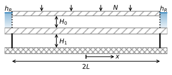
Figure 2.14 Infiltration between two rivers in a two-aquifer system.

Application of the boundary conditions ((2.52)) and ((2.53)) to the general solution ((2.40)), but using hyperbolic sine and cosine functions rather than exponential functions, results in the following solution for the head

(2.54)\[ h_0 = -\frac{N}{2T}(x^2 - L^2) - \frac{NL\lambda T_1}{TT_0}\frac{[\cosh(x/\lambda) - \cosh(L/\lambda)]}{\sinh(L/\lambda)} + h_R \]

(2.55)\[ h_1 = -\frac{N}{2T}(x^2 - L^2) + \frac{NL\lambda}{TT_0}\frac{[T_0\cosh(x/\lambda) + T_1\cosh(L/\lambda)]}{\sinh(L/\lambda)} -\frac{N\lambda^2}{T_0}+ h_R \]

The corresponding discharge vector in the two aquifers is

(2.56)\[ Q_{x_0} = -T_0\frac{\text{d} h_0}{\text{d}x} = \frac{T_0 N x}{T} + \frac{NLT_1 \sinh(x/\lambda)}{T\sinh(L/\lambda)} \]

(2.57)\[ Q_{x_1} = -T_1\frac{\text{d} h_1}{\text{d}x} =\frac{T_1 N x}{T} - \frac{NLT_1 \sinh(x/\lambda)}{T\sinh(L/\lambda)} \]

As an example, the head and flow in the two-aquifer system are simulated for the case that the leakage factor \(\lambda\) is equal to 20% of the distance between the two rivers (\(2L=5\lambda\)). The head is also simulated with a single-aquifer model, using the solution of Section 1.2. The head in the top aquifer of the two-aquifer model is smaller than the head in the single-aquifer model (Figure 2.15). The relative difference is at most 27% for the values used below. Water that infiltrates in the center part of the system flows partly through the bottom aquifer on its way to the river.

# parameters
hR = 0 # head in river, m
N = 0.001 # recharge, m/d
L = 500 # half distance between two rivers, m
k0 = 10 # hydraulic conductivity aquifer 0, m/d
H0 = 10 # thickness aquifer 0, m
k1 = 20 # hydraulic conductivity aquifer 1, m/d
H1 = 10 # thickness aquifer 1, m
kstar = 0.005 # hydraulic conductivity leaky layer, m/d
Hstar = 3 # thickness leaky layer, m
T0 = k0 * H0 # transmissivity aquifer 0, m^2/d
T1 = k1 * H1 # transmissivity aquifer 1, m^2/d
T = T0 + T1
c = Hstar / kstar # resistance leaky layer, d
lab = np.sqrt(c * T0 * T1 / (T0 + T1)) # leakage factor
print(f'leakage factor: {lab:.0f} m')

leakage factor: 200 m

# solution head
x = np.linspace(-L, L, 401)
h0 = -N / (2 * T) * (x ** 2 - L ** 2) - N * L * lab * T1 / (T * T0) * (
     np.cosh(x / lab) - np.cosh(L / lab)) / np.sinh(L / lab) + hR
h1 = -N / (2 * T) * (x ** 2 - L ** 2) + N * L * lab  / (T * T0) * (
     T0 * np.cosh(x / lab) + T1 * np.cosh(L / lab)) / np.sinh(L / lab) -\
     N * lab ** 2 / T0 + hR
h = -N / (2 * T0) * (x ** 2 - L ** 2) + hR # single layer solution, Section 1.2
print('relative diff in head at center between single layer and two-layer sol:',
      f'{(h[200] - h0[200]) / h0[200]:.2f}')
# solution Qx
xg = np.linspace(-L, L, 400)
Qx0 = T0 * N * xg / T + N * L * T1 * np.sinh(xg / lab) / (T * np.sinh(L / lab))
Qx1 = T1 * N * xg / T - N * L * T1 * np.sinh(xg / lab) / (T * np.sinh(L / lab))
Qx = N * xg
# solution stream function
zg = [-H0 - Hstar - H1, -H0 - Hstar, -H0, 0]
psi = np.zeros((4, len(xg)))
psi[1] = Qx1
psi[2] = Qx1
psi[3] = Qx1 + Qx0

relative diff in head at center between single layer and two-layer sol: 0.27

# basic plot
plt.subplot(121)
plt.plot(x, h0, label='aquifer 0')
plt.plot(x, h1, label='aquifer 1')
plt.plot(x, h, 'k--', label='single aquifer')
plt.legend()
plt.subplot(122)
plt.plot(xg, Qx0, label='aquifer 0')
plt.plot(xg, Qx1, label='aquifer 1')
plt.plot(xg, Qx, 'k--', label='single aquifer');

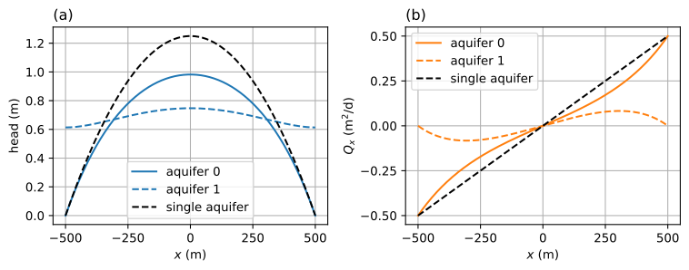
Figure 2.15 Infiltration between two rivers in a two-aquifer system; head (left) and \(Q_x\) (right).

The head in the top aquifer and streamlines in a vertical cross section are shown in Figure 2.16

# basic streamline plot
plt.contour(xg, zg, psi, 40);

Figure 2.16 Head in the top aquifer and streamlines in a vertical cross-section for infiltration between two rivers in a two-aquifer system. Discharge between two streamlines is \(\Delta\psi=0.025\) m\(^2\)/d.

      The difference between a single-layer model with an impermeable base and a two-aquifer model increases when the leakage factor \(\lambda\) decreases compared to the distance \(L\) between the two rivers. The leakage factor increases when, for example, the resistance \(c\) of the leaky layer is larger or when the transmissivity of the bottom aquifer is larger, as can be seen from Eq. (2.38). In the figure below, the head halfway the two rivers \((x=0)\) in the top aquifer is plotted for different values of the leakage factor (Figure 2.17). The dashed line represents the head at the center of the aquifer when the bottom of the top aquifer is approximated as impermeable.

lablist = np.linspace(100, 1000, 100)
hcenter = np.zeros(len(lablist))
for i, lab in enumerate(lablist):
    hcenter[i] = N / (2 * T) * L ** 2 - N * L * lab * T1 / (T * T0) * (
                 1 - np.cosh(L / lab)) / np.sinh(L / lab) + hR

# basic plot
plt.plot(lablist, hcenter)
plt.axhline(N * L ** 2 / (2 * T0), color='k', ls='--');

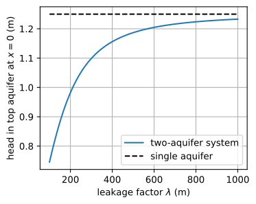
Figure 2.17 Head halfway the two rivers \((x=0)\) in the top aquifer as a function of the leakage factor, and the head for a single aquifer with an impermeable base.

Exercise 2.5

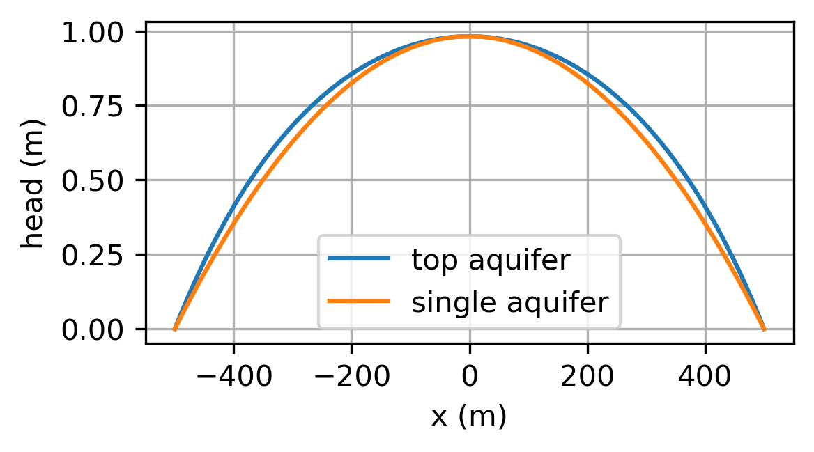
Compare the single-aquifer solution with an impermeable base to the two-aquifer solution using \(\lambda=200\) m. Compute the effective transmissivity of the single-aquifer solution such that the head at \(x=0\) is the same as the head at \(x=0\) in the two-aquifer solution. Plot in one graph the head vs. \(x\) in the single aquifer using the effective transmissivity and the head vs. \(x\) in the top aquifer of the two-aquifer solution.

Solution

\(T_\text{eff}=127.3\) m\(^2\)/d