8.3. Area-sinks for modeling areal recharge

Bounded areas with a specified flux are called area-sinks. Area-sinks are the last type of analytic element that is added to the analytic element code developed in this chapter. All analytic element classes Model, Element, HeadEquation, Constant, UniformFlow, Well, HeadWell, LineSink, and HeadLineSink, defined in the previous sections, are required to run the examples in this section.
     In this section, circular area-sinks are discussed with a uniform recharge. Rectangular area-sinks or area-sinks bounded by an arbitrary closed polygon also exist (e.g., Strack, 2017), but their equations are significantly more complicated and beyond the scope of this book. Circular area-sinks are very useful for the simulation of areal recharge from precipitation. Their circular geometry is commonly not a problem as long as the area-sink covers the entire model area, and heads are fixed inside the model area by, e.g., head-specified line-sinks, as shown in the example at the end of this section.
     Consider a circular area-sink of radius \(R\) and centered at \((x,y)=(x_a,y_a)\). Inside the area-sink, the recharge is uniform and equal to \(N\). Note that \(N\) is positive for water entering the aquifer (this is opposite to wells and line-sinks where the discharge \(Q\) and discharge per unit length \(\sigma\) are positive for water leaving the aquifer). The governing differential equation inside the area-sink is

(8.10)\[ \nabla^2 \Phi = \frac{\text{d}^2\Phi}{\text{d} r^2}+\frac{1}{r}\frac{\text{d}\Phi}{\text{d} r}= -N {\hskip 2em} r \le R \]

where \(r=\sqrt{(x-x_a)^2 + (y-y_a)^2}\) is a local radial coordinate. The areal recharge equals zero outside the area-sink, where the governing differential equation is Laplace’s equation. The solution inside the area-sink was already derived in Section 6.1

(8.11)\[ \Phi = -\frac{1}{4}N (r^2-R^2) {\hskip 2em} r\le R \]

Outside the area-sink, the solution is equal to the solution for an injection well with injection rate \(N\pi R^2\) and zero potential at \(r=R\)

(8.12)\[ \Phi = -\frac{NR^2}{2}\ln(r/R) {\hskip 2em} r\ge R \]

Note that the potential (and hence the head) and the discharge vector are continuous across the edge of the area-sink.
     The AreaSink class is defined below. Input arguments are the model that the area-sink is added to, the location of the center of the area-sink, the uniform recharge inside the area-sink, and the radius of the area-sink. The AreaSink class stores all input arguments and includes the potinf function defined above as ((8.11)) and ((8.12)) with \(N=1\).

class AreaSink(Element):
    
    def __init__(self, model, xc=0, yc=0, N=0.001, R=100):
        Element.__init__(self, model, N)
        self.xc, self.yc = xc, yc
        self.R = R
            
    def potinf(self, x, y):
        r = np.sqrt((x - self.xc) ** 2 + (y - self.yc) ** 2)
        r = np.where(r == 0, 1e-12, r)
        phi = np.where(r < self.R, 
                       -0.25 * (r ** 2 - self.R ** 2),
                       -self.R ** 2 / 2 * np.log(r / self.R))
        return phi

     As a first example, consider the synthetic case of two area-sinks next to each other. One is a recharge area, the other is a discharge area. The total amount of recharge is equal to the total amount of discharge, so that the flow field is symmetric and the problem can be used to verify the implementation of the solution. Contours of the head are shown on the left and a cross-section through the centers of the two area-sinks is shown on the right of Figure 8.7 . Note that the highest and lowest heads are not at the centers of the area-sinks.

# parameters and model
ml = Model(T=100) # transmissivity, m^2/d
rf = Constant(ml, xc=0, yc=0, hc=20)
as1 = AreaSink(ml, xc=-500, yc=0, N=0.001, R=500) # recharge, m/d
as2 = AreaSink(ml, xc=500, yc=0, N=-0.001, R=500) # discharge, m/d

# solution
ml.solve()
xg, yg = np.meshgrid(np.linspace(-1500, 1500, 100), np.linspace(-800, 800, 101))        
h = ml.head(xg, yg)

# basic plot
plt.subplot(121, aspect=1)
plt.contour(xg, yg, h, 20)
plt.subplot(122)
plt.plot(xg[0], h[50]);

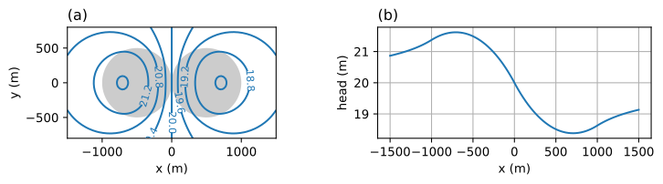
Figure 8.7 Two circular area-sinks; head contours (left) and head along \(x\)-axis (right).

Exercise 8.6

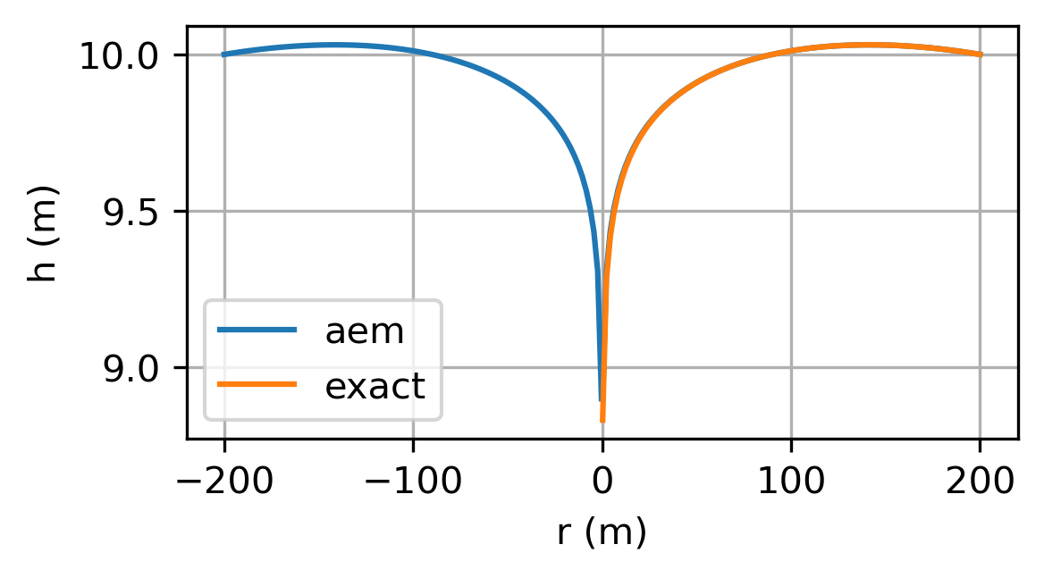
Replicate the final example of Section 6.1 using analytic elements for the case that the well pumps half the recharge on the island. Approximate the transmissivity as \(k(h_R-z_b)\). Plot the analytic element solution with constant transmssivity and the exact solution for unconfined flow of Section 6.1 on the same graph.

Solution

     As a final example, all analytic elements are combined in one model with two pumping wells located between two river branches. Each river branch is simulated with 8 line-sinks. The locations and discharges of the wells, and the coordinates and heads at the centers of the river segments, are given below and plotted in Figure 8.8 (left graph). Areal recharge is added with a circular area-sink that is large enough to cover the area between the rivers.
     The head is specified at a point outside the model area; such a point is called the reference point in analytic element models. The specified head at the reference point controls how much water flows from infinity towards the model area. A lot of water flows towards the model area when the head at the reference point is high, while water flows away from the model area towards infinity when the head at the reference point is low. As such, the reference point is a model feature and not a physical feature. The head at the reference point does not affect the head in the model area significantly if the model area is surrounded by enough head-specified elements (e.g., rivers, streams, canals). It is recommended to specify a head at the reference point such that the head gradients outside the modeled area are similar to the head gradients inside the model area.

# river segments, all in m
xls0 = [0, 100, 200, 400, 600, 800, 1000, 1100, 1200]
yls0 = [200, 200, 100, 100, 0, 0, 100, 300, 450]
hls0 = np.linspace(39, 40.4, 8)
xls1 = [0, 0, 200, 400, 600, 800, 1000, 1100, 1200]
yls1 = [200, 400, 600, 600, 700, 700, 750, 800, 850]
hls1 = np.linspace(39, 40.4, 8)

# parameters and model
ml = Model(T=100) # transmissivity, m^2/d
rf = Constant(ml, xc=0, yc=800, hc=39.5)
w0 = Well(ml, xw=500, yw=250, Q=100) # discharge, m^3/d
w1 = Well(ml, xw=800, yw=500, Q=100) # discharge, m^3/d
for i in range(len(hls0)):
    HeadLineSink(ml, xls0[i], yls0[i], xls0[i + 1], yls0[i + 1], hls0[i])
for i in range(len(hls1)):
    HeadLineSink(ml, xls1[i], yls1[i], xls1[i + 1], yls1[i + 1], hls1[i])
ar = AreaSink(ml, xc=600, yc=400, N=0.001, R=700) # recharge, m/d

# solution
ml.solve()
xg, yg = np.meshgrid(np.linspace(-100, 1300, 100), np.linspace(-100, 900, 100))
h = ml.head(xg, yg)

# basic contour plot (right side of figure)
plt.subplot(111, aspect=1)
cs = plt.contour(xg, yg, h, np.arange(38, 41, 0.2), colors='C0')
plt.clabel(cs, fmt='%1.1f', fontsize='smaller')
plt.contour(xg, yg, h, np.arange(38.1, 41, 0.2), colors='C0')
plt.plot(xls0, yls0, 'k')
plt.plot(xls1, yls1, 'k')
plt.plot([w0.xw, w1.xw], [w0.yw, w1.yw], 'k.');

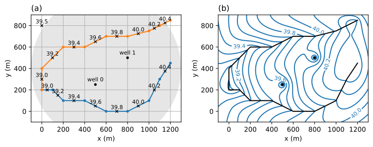
Figure 8.8 Example with wells, line-sinks, an area-sink, and a reference point; layout (left) and head contours (right).