7.5. Two wells in uniform background flow

The discharge potential and stream function for groundwater flow problems governed by Laplace’s equation (i.e., steady flow and negligible areal infiltration) may be combined into a complex potential, because the potential and stream function fulfill the Cauchy-Riemann conditions ((6.17)) (Strack, 1989). The real part of the complex potential \(\Omega\) is the discharge potential and the imaginary part is the stream function

(7.29)\[ \Omega = \Phi + i\Psi \]

In mathematical terms, this means that the stream function is the harmonic conjugate of the discharge potential (Strack, 1989). The complex potential \(\Omega\) is a function of the complex coordinate \(\zeta=x+iy\), where \(i\) is the imaginary unit (\(i^2=-1\)). The letter j is used for the imaginary unit in Python, but \(i\) is used in the mathematical equations in this book. The negative derivative of the complex potential is the complex discharge

(7.30)\[ W(\zeta)=-\frac{\text{d} \Omega}{\text{d}\zeta} = Q_x-iQ_y \]

Note that the imaginary part of the complex discharge is minus the component of the discharge vector in the \(y\)-direction.
      The introduction of complex variables makes it easy to compute the discharge potential and stream function simultaneously and allows for the use of sophisticated tools, including conformal mapping, to solve groundwater flow problems. More information on the application of complex variables in solving groundwater flow problems can be found in, e.g., Polubarinova-Kochina (1962), Harr (1962), Verruijt (1970), and Strack (1989).
      The complex potential for uniform flow is

(7.31)\[ \Omega = -W_u \zeta \]

where \(W_u\) is the uniform complex discharge

(7.32)\[ W=W_u = U - iV \]

The complex potential for a well is

(7.33)\[ \Omega = \frac{Q}{2\pi}\ln(\zeta-\zeta_w) \]

where \(Q\) is the discharge of the well and \(\zeta_w=x_w + iy_w\) is the complex coordinate of the well location. The validity of ((7.33)) is shown by writing \(\zeta-\zeta_w\) in polar form

(7.34)\[ \zeta - \zeta_w = r\text{e}^{i\theta} \]

where \(r\) is the distance between \(\zeta\) and \(\zeta_w\) and \(\theta\) is the angle that a vector pointing from \(\zeta_w\) to \(\zeta\) makes with the positive \(x\)-direction. Substitution of ((7.34)) for \(\zeta-\zeta_w\) in ((7.33)) gives

(7.35)\[ \Omega = \frac{Q}{2\pi}\ln(r\text{e}^{i\theta}) = \frac{Q}{2\pi}\ln(r) + i\frac{Q}{2\pi}\theta \]

which means that the real part of \(\Omega\) is indeed equal to the discharge potential for a well ((6.37)) and the imaginary part is equal to the stream function ((6.41)). The corresponding complex discharge for a well is

(7.36)\[ W = -\frac{\text{d}\Omega}{\text{d}\zeta}= -\frac{Q}{2\pi}\frac{1}{\zeta-\zeta_w} \]

The complex potential for \(N\) wells in uniform background flow is obtained through superposition of ((7.31)) and ((7.33)) as

\[ \Omega = -W_u \zeta + \sum_{n=1}^N\frac{Q_n}{2\pi}\ln(\zeta-\zeta_n) + C \]

where \(Q_n\) is the discharge of well \(n\), \(\zeta_n\) is the complex location of well \(n\), and an arbitrary constant \(C\) is added for completeness.
      The complex potential is applied to determine the capture zones of two wells in a field of uniform flow. The complex potential is

(7.37)\[ \Omega = -W_u \zeta + \frac{Q_0}{2\pi}\ln(\zeta-\zeta_0) + \frac{Q_1}{2\pi}\ln(\zeta-\zeta_1) + C \]

and the complex discharge function

(7.38)\[ W = W_u -\frac{Q_0}{2\pi}\frac{1}{\zeta-\zeta_0} -\frac{Q_1}{2\pi}\frac{1}{\zeta-\zeta_1} \]

The stagnation points are found by setting \(W=0\), which gives, after multiplication with \(2\pi(\zeta-\zeta_0)(\zeta-\zeta_1)\) and canceling terms

(7.39)\[ 2\pi W_u(\zeta-\zeta_0)(\zeta-\zeta_1) -Q_0(\zeta-\zeta_1) -Q_1(\zeta-\zeta_0) = 0 \]

This is a second order polynomial in \(\zeta\), which may be rearranged to give

(7.40)\[ 2\pi W_u\zeta^2 - (Q_0+Q_1+2\pi W_u(\zeta_0+\zeta_1))\zeta + Q_0\zeta_1 + Q_1\zeta_0 + 2\pi W_u\zeta_0\zeta_1 = 0 \]

The complex locations of the stagnation points may now be found with standard equations for the roots of a second order polynomial. Note that application of the complex potential makes it possible to compute the locations of the stagnation points quite easily even when the wells are at arbitrary locations and the uniform flow is in an arbitrary direction. The procedure may be extended to an arbitrary number of wells as shown in Bakker (2025).
      As an example, the capture zone envelopes of the two wells of Figure 7.5 are computed. After the stagnation points are computed, the capture zone envelopes can be plotted. The streamplot function is used to compute and plot the capture zone envelopes, because contouring the stream function results in a figure with two ugly branch cuts. Two pathlines are started from each stagnation point, one slightly to the left of a stagnation point and one slightly to the right of a stagnation point. The pathlines are integrated in both directions (the default in streamplot) to create the two boundaries of a capture zone envelope.

# parameters
Wu = 1.2 + 0j # complex uniform flow, m^2/d
Q0, Q1 = 500, 500 # discharge of wellw, m^3/d
zeta0, zeta1 = 0 + 0j, 100 + 100j # complex locations of wells, m

# solution
a = 2 * np.pi * Wu
b = -(Q0 + Q1 + 2 * np.pi * Wu * (zeta0 + zeta1))
c = Q0 * zeta1 + Q1 * zeta0 + 2 * np.pi * Wu * zeta0 * zeta1
zetas0 = (-b - np.sqrt(b ** 2 - 4 * a * c)) / (2 * a)
zetas1 = (-b + np.sqrt(b ** 2 - 4 * a * c)) / (2 * a)
xs0, ys0 = zetas0.real, zetas0.imag
xs1, ys1 = zetas1.real, zetas1.imag
print(f'(x,y) stagnation point 0: {xs0:.2f}, {ys0:.2f}')
print(f'(x,y) stagnation point 1: {xs1:.2f}, {ys1:.2f}')

(x,y) stagnation point 0: 41.96, 16.38
(x,y) stagnation point 1: 190.67, 83.62

Alternatively, if you don’t want to program the equation for the roots of a polynomial, you can use the Polynomial class of the numpy.polynomial package. The Polynomial class takes the coefficients of the polynomial as inputs (from low to high order), and the roots function returns the roots.

from numpy.polynomial import Polynomial
poly = Polynomial([c, b, a])
print('stagnation points:', poly.roots())

stagnation points: [ 41.96276198+16.37606515j 190.66635726+83.62393485j]

Finally, functions for the complex potential and discharge function are defined and the capture zones are drawn.

# functions for complex potential and complex discharge function
def omega(x, y):
    zeta = x + y * 1j
    om = -Wu * zeta + Q0 / (2 * np.pi) * np.log(zeta - zeta0) + Q1 / (2 * np.pi) * np.log(zeta - zeta1)
    return om

def wdis(x, y):
    zeta = x + y * 1j
    W = Wu - Q0 / (2 * np.pi * (zeta - zeta0)) - Q1 / (2 * np.pi * (zeta - zeta1))
    return W

# plot of head contours and capture zone envelopes
x, y = np.meshgrid(np.linspace(-800, 200, 100), np.linspace(-300, 400, 100))
om = omega(x, y)
w = wdis(x, y)
Qx, Qy = w.real, -w.imag
plt.subplot(111, aspect=1)
plt.contour(x, y, om.real, 10, colors='C0')
plt.streamplot(x, y, Qx, Qy, start_points=np.array([(xs0 + 1, ys0), (xs0 - 1, ys0)]), 
               density=100, color='C1')
plt.streamplot(x, y, Qx, Qy, start_points=np.array([(xs1 + 1, ys1), (xs1 - 1, ys1)]), 
               density=100, color='C2')
plt.plot([zeta0.real, zeta1.real], [zeta0.imag, zeta1.imag], 'k.')

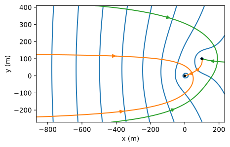
Figure 7.9 Capture zone envelopes for two wells in a uniform background flow for the same problem as Figure 7.5.

Exercise 7.9

Repeat Exercise 7.4 but with complex variables.

Exercise 7.10

Repeat Exercise 7.7 but with complex variables.